How AI Works · 14 min read
The Model Was Wrong. Which Weight Should We Blame?
A slow, number-by-number journey through backpropagation—from a loss of 0.782 to gradients, updated weights and a better second prediction.
Following one error backward through a neural network
A note on the headline: The model selects the correct word, blue, in this example. “Wrong” refers to the remaining prediction loss, not an incorrect top-ranked answer. A gradient measures local sensitivity with other parameters held fixed; “blame” and “responsibility” are teaching metaphors, not a unique division of the total error among weights. Displayed arithmetic is rounded; run the code at full precision to reproduce the results.
This is the second article in our three-part journey:
Forward pass → Backpropagation → Gradient descentThe forward pass gave us a prediction and a loss. We will now find how much each trainable number contributed to that loss.
In the previous article, we gave a tiny neural network this incomplete sentence:
The sky is …
It had three possible next words:
blue
green
runs
After one forward pass, the network produced:
| Token | Raw score | Probability |
|---|---|---|
blue | 0.84 | 45.73% |
green | 0.67 | 38.58% |
runs | -0.23 | 15.69% |
The correct answer was blue, and the model did select it.
But 45.73% is hardly confidence. The model nearly chose green.
Cross-entropy turned that uncertainty into one number:
Now we have a problem.
The network contains several weights and biases. The final loss only says
0.782. It does not directly tell us:
- which weight helped the correct answer;
- which weight pushed the model toward a wrong answer;
- how strongly each parameter affected the loss;
- or how much each parameter should change.
This is the job of backpropagation.
Backpropagation takes the final error and traces responsibility backward, operation by operation, until every trainable parameter receives a gradient.
flowchart RL
    Loss["Loss: 0.782"] --> Scores["Output scores"]
    Scores --> Hidden["Hidden values"]
    Hidden --> First["Earlier weights"]
The diagram points backward, but nothing literally travels through the network. We are calculating how sensitive the loss is to each earlier number.
By the end of this article, we will update every weight once and run the model
again. The probability of blue will rise from 45.73% to 56.44%, while the
loss will fall from 0.782 to 0.572.
Let us see exactly why.
First, what does “learning” mean here?
A neural network learns by changing its parameters so that future predictions produce a smaller loss.
One training step has four stages:
flowchart TD
    Forward["1. Make prediction"] --> Loss["2. Measure loss"]
    Loss --> Backward["3. Calculate gradients"]
    Backward --> Update["4. Update parameters"]
    Update --> Again["Run again"]
The forward pass completed the first two stages. This article focuses on stages three and four.
Backpropagation does not update the weights. It calculates the gradients. An optimizer—using a rule such as gradient descent—uses those gradients to update the weights.
That distinction matters:
backpropagation → finds the direction and sensitivity
optimizer       → decides the actual parameter update
You can think of backpropagation as a diagnostic report and the optimizer as the mechanic who acts on it.
Meet the same network again
The text has already been represented by a small teaching vector:
The first layer uses these parameters:
The forward calculation was:
ReLU kept both positive values:
The output layer uses:
It produced:
Softmax converted those logits into:
The target vector for blue is:
This is called one-hot encoding. The 1 marks the correct class; the zeros
mark the incorrect classes.
During the forward pass, the network saved intermediate values such as x,
z, h, logits and probabilities. Backpropagation will need them.
Before the arithmetic: what is a gradient?
Suppose one weight is currently 0.4.
If slightly increasing it makes the loss increase, that weight’s gradient is positive. If slightly increasing it makes the loss decrease, its gradient is negative.
The notation
means:
If I change weight by a tiny amount, how does loss respond?
For example:
roughly says that a tiny increase of 0.01 in the weight would increase the
loss by about:
If instead:
the same tiny increase would reduce the loss by about 0.02.
The gradient therefore gives us two useful pieces of information:
| Gradient | Direction | Sensitivity |
|---|---|---|
| Positive | Increasing the parameter raises loss | Magnitude tells us how strongly |
| Negative | Increasing the parameter lowers loss | Magnitude tells us how strongly |
| Near zero | Small local effect on loss | Parameter may barely change |
A gradient is not the amount by which we automatically change a weight. It is a local slope. The optimizer combines that slope with a learning rate.
A quick numerical way to feel a gradient
Suppose a weight is 0.4000 and the current loss is 0.782381.
We increase the weight by a tiny amount:
weight: 0.4000 → 0.4001Imagine that the loss becomes approximately 0.782316. The loss changed by:
Divide by the weight change:
That is close to the analytical gradient -0.6512 we will calculate for this
weight. This technique is called a finite-difference check. It is slower and
less precise than backpropagation, but it gives us a concrete interpretation:
slightly increasing this weight makes the loss slightly smaller.
Why travel backward?
Our loss depends on the probability of blue. That probability depends on all
three logits. The logits depend on the hidden values. The hidden values depend
on ReLU outputs. Those depend on the first layer’s weights and biases.
flowchart TD
    P1["W₁ and b₁"] --> H["Hidden values"]
    H --> P2["W₂ and b₂"]
    P2 --> O["Logits"]
    O --> L["Loss"]
The forward pass follows the arrows downward. To find how W₁ affected the
loss, we must follow the dependency path in reverse.
This is where the chain rule enters.
If depends on , and depends on , then:
In plain language:
Effect of
bon the loss = effect ofbon the next value × effect of that next value on the loss.
Backpropagation is the chain rule applied repeatedly and efficiently across the network’s computation graph.
Start where the error is easiest to see
We used softmax followed by cross-entropy. Together, they give us a pleasantly simple gradient for every output logit:
We have:
and:
Subtract position by position:
These are the gradients of the loss with respect to the three logits.
| Token | Probability | Target | Logit gradient |
|---|---|---|---|
blue | 0.4573 | 1 | -0.5427 |
green | 0.3858 | 0 | +0.3858 |
runs | 0.1569 | 0 | +0.1569 |
Now interpret the signs.
The blue gradient is negative. Increasing the blue logit would reduce the
loss, so gradient descent will push that score upward.
The other gradients are positive. Increasing those logits would increase the loss, so gradient descent will push them downward.
Also notice:
Softmax classes compete with one another. Probability moved toward one class must come from somewhere else.
Assigning responsibility to the output weights
Consider the connection from hidden value to the blue logit. Its
weight is 0.4.
During the forward pass, its contribution was:
The gradient for that weight is:
Why multiply by 1.2? Because a weight connected to a large incoming value has
more influence than the same weight connected to zero.
We repeat this for every connection. In matrix form, this is an outer product:
Each cell corresponds to one output weight in the same position as .
The output bias gradients are even simpler. A bias is added directly to its logit, so:
There is no incoming activation to multiply because the derivative of
logit + bias with respect to that bias is 1.
The error now reaches the hidden layer
The output layer has received its gradients, but we are not finished. The hidden values also influenced all three logits.
For the first hidden value:
For the second hidden value:
Together:
This is another dot-product calculation. Each hidden value fans out to three outputs, so its responsibility is the sum of all three paths.
One important detail: we used the old values here. All gradients for one backward pass must describe the same forward pass. Updating weights halfway through would mix two different versions of the network.
Backward through ReLU
During the forward pass:
ReLU’s local derivative is:
At exactly , the mathematical derivative is not uniquely defined. Software frameworks choose a convention—commonly zero—for the backward pass. Our two values are positive, so that edge case does not affect this example.
Both pre-activation values were positive:
So both local derivatives are 1:
The symbol means element-by-element multiplication.
Nothing changed in this example. But suppose the second pre-activation had been negative. ReLU would have output zero, and its local derivative would also be zero. The gradient on that path would stop there for this input.
That is why people sometimes describe ReLU as a gate:
positive during forward pass → gradient passes backward
negative during forward pass → gradient becomes zero
Reaching the first layer
We have now reached the first weighted calculation:
The input was:
As before, a weight gradient is the incoming value multiplied by the gradient arriving at its output neuron:
The bias gradients are:
We could also calculate a gradient for the input vector:
In a larger model, that gradient would continue into whatever earlier layer
created x—perhaps an embedding table or another Transformer block. In our
teaching network, x is the beginning, so we can stop.
Every trainable parameter now has a gradient.
The entire backward pass in one table
| Backward stage | Incoming gradient | Local operation | Result |
|---|---|---|---|
| Softmax + loss | Target and probabilities | ||
| Output weights | and | , shape [2,3] | |
| Output biases | Direct addition | ||
| Hidden values | and | ||
| ReLU | and saved | ReLU gate | |
| First weights | and | , shape [2,2] | |
| First biases | Direct addition |
The backward formulas may look different, but the repeated idea is simple:
Take the gradient arriving from the right, multiply by the local effect of the current operation, and pass the result farther left.
Gradients are ready. Now the optimizer acts.
We will use basic gradient descent with a learning rate of:
The update rule is:
Why subtract?
The gradient points toward increasing loss. We want to move in the opposite direction.
Take the first output weight for blue:
old weight = 0.4
gradient   = -0.6512
Update it:
The weight increased. That makes sense: its negative gradient told us that increasing this weight should reduce the loss.
Now take the first output weight for green:
old weight = 0.1
gradient = 0.4630This weight decreased because it was helping the incorrect green score.
After updating every parameter:
One optimizer step is complete.
Did the model actually improve?
Never assume an update helped. Run another forward pass and measure it.
Using the updated first layer:
Both are positive, so ReLU keeps them:
The updated output layer produces:
Softmax gives:
| Token | Before update | After update |
|---|---|---|
blue | 45.73% | 56.44% |
green | 38.58% | 30.37% |
runs | 15.69% | 13.19% |
The correct token gained probability. Both incorrect tokens lost probability.
The new loss is:
| Measurement | Before | After one update |
|---|---|---|
| Correct-token probability | 45.73% | 56.44% |
| Loss | 0.782 | 0.572 |
This is one tiny moment of learning.
The network did not memorize an English grammar rule in words. It changed numbers so that this input now creates a stronger score for the target.
One example is not complete learning
It would be misleading to say the model has “learned that the sky is blue” after one update.
Real training repeats the loop over many examples:
forward pass
→ loss
→ zero old gradients
→ backpropagation
→ optimizer update
→ next batch
After the model processes all training examples once, we call that one epoch. Training may require many epochs or, for large language models, a very large number of batches in one or more passes through enormous datasets.
The direction also changes from example to example. One sentence may push a weight upward. Another may push it downward. Useful learning emerges from the combined statistical pressure of many examples—not from blindly maximizing one answer for one sentence.
If we repeatedly trained only on The sky is → blue, the model could become
extremely confident on that example while performing poorly elsewhere. That is
memorization, not broad generalization.
What changes when training a real LLM?
The tiny network lets us inspect every number. A real Transformer may contain millions or billions of parameters and many repeated blocks.
The basic logic remains the same:
- Token embeddings enter the model.
- Attention and feed-forward layers produce hidden representations.
- The final layer produces vocabulary logits.
- Cross-entropy measures next-token error.
- Automatic differentiation traces gradients backward through every recorded operation.
- An optimizer updates the parameters.
No engineer manually writes billions of derivative calculations. Frameworks
such as PyTorch build a dynamic computation graph during the forward pass and
perform reverse-mode automatic differentiation when .backward() is called.
But automation does not change the mathematics. Under the hood, the system is still applying local derivatives and the chain rule.
Batches
Real training calculates gradients for many tokens and sequences together. Their contributions are commonly summed or averaged into one gradient for each parameter before the optimizer step.
Attention
Gradients flow backward through Value mixing, attention probabilities, softmax, Query–Key dot products and the learned projection matrices.
Shared parameters
The same parameter may be used at many token positions. Its gradient receives contributions from every path where it was used.
GPU parallelism
The workload is dominated by large matrix multiplications. GPUs perform many of these multiply-and-add operations in parallel during both forward and backward passes. Training usually requires more memory than inference because the backward pass needs saved activations, gradients and optimizer state.
The same example in Python
The following code performs the complete loop manually. It does not use an automatic differentiation library, so every backward equation remains visible.
import numpy as np


x = np.array([1.0, 2.0])
y = np.array([1.0, 0.0, 0.0])  # blue is correct

W1 = np.array([
    [0.5, -0.2],
    [0.3,  0.8],
])
b1 = np.array([0.1, -0.1])

W2 = np.array([
    [0.4, 0.1, -0.3],
    [0.2, 0.5,  0.1],
])
b2 = np.array([0.1, -0.1, 0.0])


def softmax(logits):
    shifted = logits - np.max(logits)
    exponentials = np.exp(shifted)
    return exponentials / exponentials.sum()


def forward(x, W1, b1, W2, b2):
    z = x @ W1 + b1
    h = np.maximum(z, 0.0)
    logits = h @ W2 + b2
    probabilities = softmax(logits)
    loss = -np.log(probabilities[0])
    return z, h, logits, probabilities, loss


# Forward pass
z, h, logits, probabilities, loss = forward(x, W1, b1, W2, b2)

# Backward from softmax + cross-entropy
grad_logits = probabilities - y

# Output layer
grad_W2 = np.outer(h, grad_logits)
grad_b2 = grad_logits
grad_h = grad_logits @ W2.T

# ReLU
grad_z = grad_h * (z > 0)

# First layer
grad_W1 = np.outer(x, grad_z)
grad_b1 = grad_z

# Gradient-descent update
learning_rate = 0.1
W1 -= learning_rate * grad_W1
b1 -= learning_rate * grad_b1
W2 -= learning_rate * grad_W2
b2 -= learning_rate * grad_b2

# Verify with a second forward pass
_, _, new_logits, new_probabilities, new_loss = forward(
    x, W1, b1, W2, b2
)

print("before probabilities:", probabilities)
print("before loss:", loss)
print("after probabilities:", new_probabilities)
print("after loss:", new_loss)
Expected output is approximately:
before probabilities: [0.4573, 0.3858, 0.1569]
before loss:           0.7824

after probabilities:  [0.5644, 0.3037, 0.1319]
after loss:            0.5720
Common misunderstandings
“Backpropagation moves the prediction backward”
It does not reverse the input or undo the prediction. It calculates derivatives backward through the dependency graph.
“The gradient is the error”
The loss is the error measurement. A gradient measures how sensitive that loss is to a particular value.
“A negative gradient is bad”
The sign is not a quality score. It tells us direction. A negative gradient means increasing that parameter locally reduces the loss.
“Backpropagation updates the weights”
Backpropagation calculates gradients. The optimizer applies updates.
“The learning rate is part of the gradient”
The gradient comes from the network and loss. The learning rate is a training choice controlling step size.
“A lower training loss always means a better model”
Not necessarily. The model can overfit its training data. We also evaluate on validation data it did not use for parameter updates.
“Gradients always remain healthy in deep networks”
Repeated multiplication can make gradients extremely small or extremely large. These are vanishing and exploding gradients. Residual connections, normalization, initialization choices and gradient clipping help manage them.
“We can update each layer as soon as its gradient is ready”
Not in the ordinary backward pass. Gradients must be calculated using the same parameter values that produced the forward result. The optimizer acts after the required gradients have been accumulated.
How engineers debug backward passes
When training fails, the final loss alone is not enough. Engineers inspect the gradient flow.
Useful checks include:
- Does every trainable parameter have a gradient?
- Do any gradients contain
NaNor infinity? - Are most gradient magnitudes nearly zero?
- Are gradient norms exploding?
- Was the previous batch’s gradient cleared before the next backward pass?
- Did an accidental detach operation break the computation graph?
- Are frozen parameters intentionally frozen?
- Is the loss connected to the model output?
A compact trace for our network looks like this:
| Value | Shape | Minimum gradient | Maximum gradient |
|---|---|---|---|
| Logits | [3] | -0.5427 | 0.3858 |
[2,3] | -0.7055 | 0.5016 | |
| Hidden vector | [2] | -0.2256 | 0.1001 |
[2,2] | -0.4511 | 0.2001 |
In large networks, engineers often inspect gradient norms rather than printing every number.
The one idea to carry forward
Backpropagation is not the model looking at the answer and somehow becoming smarter.
It is a precise bookkeeping system for responsibility.
Our forward pass produced:
The correct answer was represented as:
Their difference started the backward pass:
The chain rule carried that signal backward through the output weights, hidden values, ReLU and first-layer weights. Gradient descent then made a small update.
After only one training step:
P(blue): 45.73% → 56.44%
loss:     0.782 → 0.572
Then the cycle begins again—with another forward pass, another loss, another backward pass and another update.
A model learns not through one dramatic realization, but through enormous numbers of small numerical corrections.
That is backpropagation.
The gradient has now told us the direction and sensitivity. The final article asks the remaining question: how far should each parameter move? That is where gradient descent and the learning rate enter.
Sources and further reading
- PyTorch: A Gentle Introduction to torch.autograd
- PyTorch: Automatic Differentiation with torch.autograd
- PyTorch: CrossEntropyLoss
- PyTorch: SGD
- Deep Learning, Chapter 6: Deep Feedforward Networks
Continue the series
Related learning
Want to go deeper?
Continue reading

How AI Works
Before a Neural Network Can Learn, It Must Make a Prediction
A slow, number-by-number journey through one forward pass—from ‘The sky is ...’ to a prediction, a probability and a loss.
◷ 15 min read
How AI Works
How LLMs Learn: One Training Step, Explained
A complete beginner-first walkthrough of one next-token training step—from text and vectors to logits, softmax, cross-entropy, gradients, backpropagation and a real weight update.
◷ 24 min read
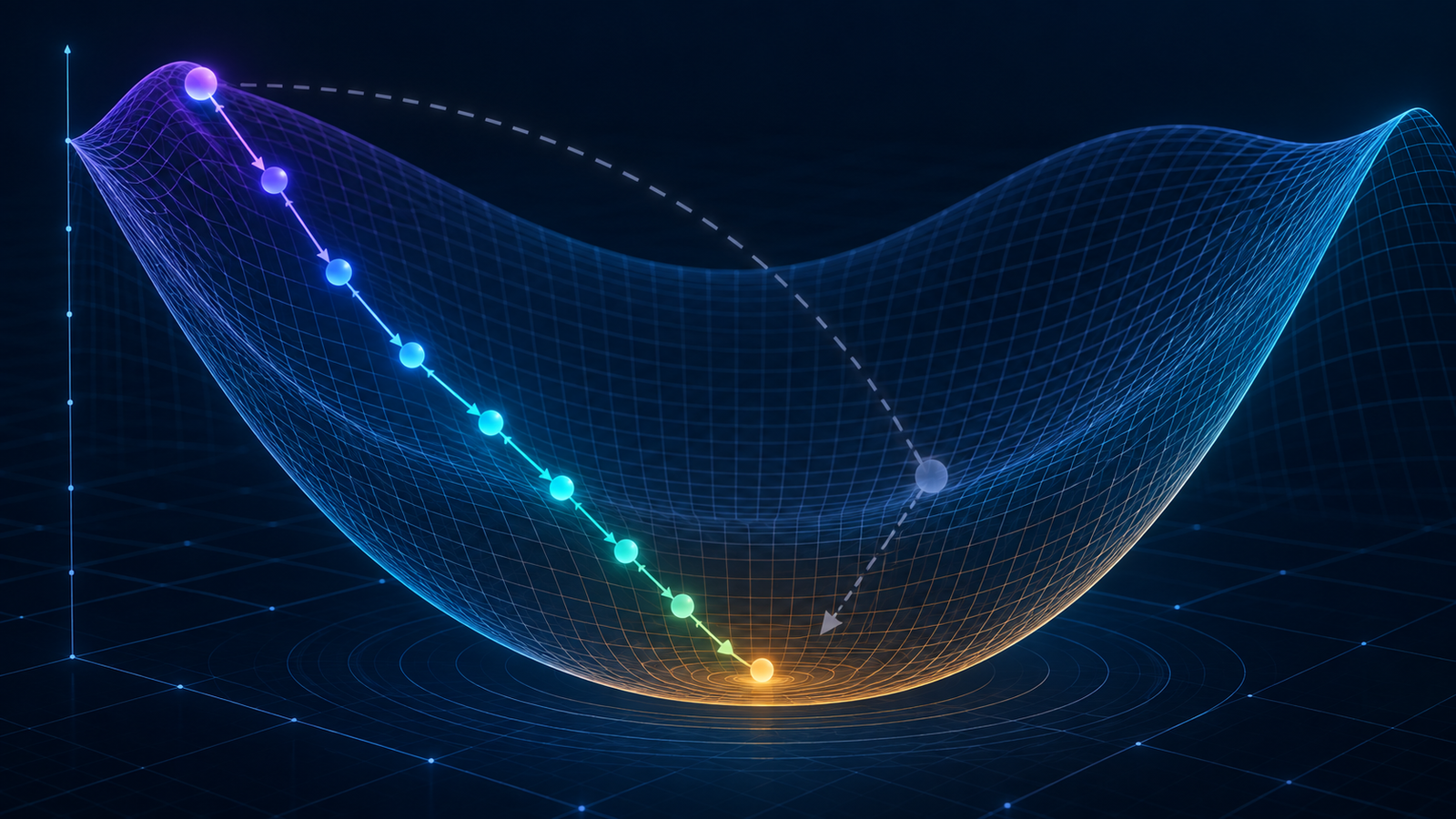
How AI Works
The Gradient Knows the Direction. But How Far Should the Model Move?
A beginner-first explanation of gradient descent, learning rates, loss landscapes, batches, momentum, Adam and AdamW—continuing our neural-network example.
◷ 14 min read