How AI Works · 24 min read
How LLMs Learn: One Training Step, Explained
A complete beginner-first walkthrough of one next-token training step—from text and vectors to logits, softmax, cross-entropy, gradients, backpropagation and a real weight update.
One Training Loop: The Moment an LLM Actually Learns
One sentence enters. One prediction is wrong. The weights move slightly. That is learning.
Suppose we want a tiny language model to learn this sentence:
The sky is blue.
We show it:
the sky isand ask:
What token should come next?
The correct answer in our training example is:
blueBut the model initially predicts:
greenWhat happens now?
The model does not receive an English correction such as:
Please understand that the sky is usually blue.
Instead, training converts the mistake into a number called loss. Calculus converts the loss into gradients. An optimizer uses those gradients to change the model’s weights by a small amount.
Then the model tries again.
Scope of this example: The worked arithmetic below updates a three-class output layer while holding the hidden state fixed. It illustrates the learning loop; it does not numerically train an entire Transformer. A single update is not guaranteed to improve every example or validation performance.
After one update, the probability of blue rises and the loss falls.
That is one complete training loop.
flowchart TD
    Data["Training text"] --> Forward["Forward pass"]
    Forward --> Prediction["Predict next token"]
    Prediction --> Loss["Measure error"]
    Loss --> Backward["Backpropagate gradients"]
    Backward --> Update["Update weights"]
    Update --> Data
This article will calculate the loop using actual numbers. Nothing important will be hidden behind “the optimizer learns.”
What does “training” mean?
A machine-learning model contains adjustable numbers called parameters.
In a neural network, the parameters are mainly:
- weights;
- and sometimes biases.
Before training, many weights are initialized to small values. The model does not yet perform the intended task reliably.
Training repeatedly does five things:
- give the model an example;
- let it make a prediction;
- measure how wrong the prediction is;
- determine which parameters contributed to the error;
- adjust those parameters slightly.
One pass through those steps is a training iteration or training step.
The phrase training loop also refers to the program that repeats these steps across batches and epochs.
Training and inference are different
When you ask a deployed LLM a question, it performs inference. It uses existing weights to generate an answer.
During training, the model also calculates gradients and updates those weights.
| Inference | Training |
|---|---|
| Receives input | Receives input and expected target |
| Performs a forward pass | Performs a forward pass |
| Produces predictions | Produces predictions |
| Usually does not calculate gradients | Calculates gradients |
| Does not normally update weights | Updates weights |
| Goal: answer | Goal: improve future predictions |
Our earlier request—“Tell me a political joke”—was inference.
Read the companion article, Inside an LLM: From Your Prompt to Its Reply, for that request’s complete journey.
This article goes back to the stage where the model’s behaviour is learned.
Part I — Preparing one training example
Step 1: begin with training text
Our tiny dataset contains one sentence:
the sky is blueA real LLM trains on vastly more text. We use four words so that every operation remains visible.
The objective is next-token prediction:
Given the earlier tokens, predict the token that comes next.
The sentence can produce several training relationships:
| Input | Target |
|---|---|
the | sky |
the sky | is |
the sky is | blue |
For our full numerical example, we will use only the last relationship:
input  = "the sky is"
target = "blue"
Step 2: tokenize the text
The tokenizer splits the text into tokens.
For this toy model:
["the", "sky", "is", "blue"]We create a tiny vocabulary:
| Token | Token ID |
|---|---|
the | 0 |
sky | 1 |
is | 2 |
blue | 3 |
green | 4 |
runs | 5 |
The training pair becomes:
input IDs  = [0, 1, 2]
target ID  = 3
Index clarification:
3is the ID ofbluein the six-token vocabulary. In the later three-candidate calculation, the local order is[blue, green, runs], sobluehas local class index0. A three-logit cross-entropy call must use target0, not vocabulary ID3.
The target ID is a category label. The number 3 does not mean that blue is three times anything.
Step 3: create input and target tensors
Frameworks store model data in tensors.
A tensor is a container of numbers with a shape.
Our input tensor contains three token IDs:
Its shape is:
[sequence length] = [3]If we train four sequences together, we might have:
[batch size, sequence length] = [4, 3]For now, our batch contains one example.
Part II — The forward pass
What is a forward pass?
The forward pass moves the input through the model to produce a prediction.
No weight is changed during this part.
flowchart LR
    IDs["Token IDs"] --> Emb["Embeddings"]
    Emb --> Net["Neural network"]
    Net --> H["Hidden state"]
    H --> Logits["Vocabulary logits"]
    Logits --> Prob["Probabilities"]
Step 4: look up token embeddings
Token IDs are row numbers in an embedding table.
Suppose our toy embeddings have two dimensions:
| Token | Embedding |
|---|---|
the | |
sky | |
is |
The input becomes a matrix:
The shape is:
[3 tokens, 2 embedding dimensions]In a real Transformer, these vectors receive positional information and pass through many attention and feed-forward layers.
Step 5: produce a contextual hidden state
Attention allows each token position to incorporate information from allowed earlier positions. Many Transformer blocks repeatedly transform those representations.
To keep this article focused on the complete training loop, we will treat those internal Transformer calculations as a function:
Suppose the final hidden state used to predict the next token is:
This is an invented two-dimensional value.
A real LLM would use a much larger hidden vector. Backpropagation will eventually continue through this hidden state, all Transformer layers and the embedding table. We will calculate that direction later.
For now, summarizes what the model currently represents about:
the sky isStep 6: convert the hidden state into logits
The model needs one score for every possible next token.
To make the arithmetic manageable, suppose only three candidate tokens are considered in our demonstration:
blue, green, runsEach candidate has an output weight vector:
The logit for a candidate is the dot product between hidden state and that candidate’s weight vector.
Logit for blue
Logit for green
Logit for runs
The logits are:
The highest score belongs to green.
The model is currently wrong.
What exactly is a logit?
A logit is an unrestricted raw score.
It can be:
- positive;
- negative;
- larger than 1;
- smaller than 0.
Logits are not probabilities and do not need to sum to 1.
The important property is relative order: a higher logit means the model favours that token more strongly before normalization.
Step 7: use softmax to create probabilities
Softmax converts the logits into positive probabilities that sum to 1.
First calculate the exponentials:
Add them:
Now divide each value by the total.
Probability of blue
Probability of green
Probability of runs
The distribution is approximately:
| Candidate | Probability |
|---|---|
blue | 32.4% |
green | 43.7% |
runs | 24.0% |
Rounding makes the displayed total 100.1%; the unrounded values sum to 1.
The model assigned only 32.4% probability to the correct answer.
Part III — Measuring the mistake
Step 8: represent the correct target
Our correct token is blue.
As a one-hot vector across the three candidates:
This means:
blueis correct: 1;greenis not the target: 0;runsis not the target: 0.
The model predicted:
We need one number measuring how poorly this prediction matches the target.
Step 9: calculate cross-entropy loss
For one correct class, cross-entropy reduces to:
The correct token’s probability is 0.324:
Rounding note: Using the unrounded softmax probability, approximately
0.323554, gives loss1.128390. Using the displayed rounded probability0.324gives1.127012. The worked example and repeated-run table use unrounded probabilities internally; intermediate displays are rounded.
The loss is approximately:
What does 1.128 mean?
It is not “1.128 wrong words.”
It is a penalty derived from how little probability the model assigned to the correct token.
Compare:
| Probability assigned to correct token | Cross-entropy loss |
|---|---|
| 0.99 | 0.010 |
| 0.80 | 0.223 |
| 0.50 | 0.693 |
| 0.10 | 2.303 |
| 0.01 | 4.605 |
Higher confidence in the correct token produces lower loss. Confidently assigning it almost no probability produces a large penalty.
Why use logarithms?
The logarithm gives useful behaviour:
- it strongly penalizes confident wrong predictions;
- losses across token positions can be added or averaged conveniently;
- it works cleanly with the probabilistic objective of maximum likelihood;
- its derivative combines elegantly with softmax.
The model’s training goal is to reduce average loss across many examples—not to force the loss of one example instantly to zero.
Part IV — Backpropagation
What question does backpropagation answer?
We know the loss is 1.128.
But the model may contain millions or billions of parameters.
Which parameters should change?
In which direction?
By how much?
Backpropagation uses the chain rule from calculus to calculate how sensitive the loss is to each parameter.
That sensitivity is a gradient.
Read this as:
If weight changes slightly, how does the loss change?
A hill analogy for gradients
Imagine standing on a foggy hill.
Height represents loss.
- Higher ground = worse loss.
- Lower ground = better loss.
The gradient points in the direction of steepest increase. To reduce the loss, move in the opposite direction.
flowchart LR
    High["Current weights: higher loss"] -->|"move opposite gradient"| Low["Updated weights: lower loss"]
One update is one small downhill step.
Step 10: calculate gradients with respect to logits
Softmax followed by cross-entropy has a remarkably clean derivative:
In words:
logit gradient = predicted probability − correct target
Our prediction is:
Our target is:
Subtract:
Gradient for blue
Gradient for green
Gradient for runs
Therefore:
Because of rounding, these displayed gradients sum to approximately 0.001 instead of exactly zero.
Interpreting the signs
bluehas a negative logit gradient. Gradient descent will increase its logit.greenhas a positive gradient. Gradient descent will reduce its logit.runsalso has a positive gradient. Its logit will be reduced.
The mathematics already expresses the correction we want.
Step 11: calculate gradients for the output weights
Each logit was calculated as:
The gradient of the loss with respect to a candidate weight vector is:
Our hidden state is:
Gradient for blue weights
Gradient for green weights
Gradient for runs weights
We now have a direction for every displayed output weight.
Step 12: continue the gradient into the hidden state
The output weights are not the only learnable parameters.
The loss also depends on hidden state , which depends on the Transformer blocks, which depend on earlier hidden states and token embeddings.
The gradient with respect to is:
Using the original weights:
First dimension:
Second dimension:
Therefore:
This gradient flows backward into the function that produced .
flowchart RL
    Loss["Loss"] --> Output["Output projection"]
    Output --> BlockN["Last Transformer block"]
    BlockN --> Blocks["Earlier blocks"]
    Blocks --> Emb["Token embeddings"]
Inside a real Transformer, automatic differentiation continues through:
- feed-forward layers;
- activation functions;
- normalization;
- residual paths;
- attention’s weighted sums;
- softmax attention weights;
- Query, Key and Value projections;
- positional operations;
- token embeddings.
The chain rule connects the final loss to every parameter that influenced it.
Does backpropagation move backward through time?
Not physically.
The forward pass builds a computational graph recording how outputs depend on earlier operations. The backward pass visits that dependency graph in reverse order to apply the chain rule.
Forward:
weights → logits → probabilities → loss

Backward:
loss gradient → probability/logit gradients → weight gradients
“Backward” describes the direction through dependencies, not a reversal of time.
Part V — Updating the weights
Step 13: choose a learning rate
The gradient tells us direction and sensitivity. We still need to decide the step size.
That step size is controlled by the learning rate.
For our example:
This is intentionally large enough to make the numerical change visible. Real training chooses learning rates through careful experimentation and scheduling.
Step 14: apply gradient descent
The basic update rule is:
We subtract the gradient because the gradient points uphill and we want lower loss.
Update blue
Old weight:
Gradient:
Update:
Subtracting a negative gradient increased both values.
Update green
Update runs
The correct token’s output weights moved in a direction that raises its compatibility with . Incorrect candidates moved in directions that lower theirs.
What if the learning rate is wrong?
Too small
The model improves very slowly and training wastes computation.
Too large
Updates can overshoot useful regions. Loss may oscillate, grow or become numerically unstable.
Appropriate
Training makes meaningful progress without becoming unstable.
Modern LLM training uses more advanced optimizers such as Adam or AdamW, learning-rate warmup, decay schedules, gradient clipping and many other controls. Basic gradient descent gives us the central idea without hiding it.
Part VI — Check whether the update helped
Step 15: run the forward calculation again
Keep the same teaching hidden state:
In a fully updated network, could also change because earlier parameters would be updated. Holding it fixed lets us isolate the effect of the output-weight update.
New blue logit
New green logit
Arithmetic note: The displayed rounded weights give
0.0563 + 2 × 0.2126 = 0.4815, which rounds to0.482. With full-precision gradients, the new logit is approximately0.481624.
New runs logit
Before the update:
blue  = 0.4
green = 0.7  ← highest
runs  = 0.1
After the update:
blue  = 0.738 ← highest
green = 0.482
runs  = -0.020
The correct token now has the highest logit.
Step 16: calculate the new probabilities
Apply softmax to:
Approximate exponentials:
Total:
New probabilities:
| Candidate | Before update | After update |
|---|---|---|
blue | 32.4% | 44.6% |
green | 43.7% | 34.5% |
runs | 24.0% | 20.9% |
One step increased the correct token’s probability from approximately 32.4% to 44.6%.
Step 17: calculate the new loss
Compare:
old loss = 1.128
new loss = 0.808
The loss decreased.
The update helped this example.
flowchart LR
    Before["Before: P(blue)=32.4%, loss=1.128"] --> Update["One gradient update"]
    Update --> After["After: P(blue)=44.6%, loss=0.808"]
The model has not “mastered the colour of the sky.” It has made one small parameter adjustment based on one example.
Part VII — One full loop in a table
| Stage | Input | Operation | Output |
|---|---|---|---|
| 1 | the sky is blue | Tokenize | Token sequence |
| 2 | Tokens | Map through vocabulary | Input IDs and target ID |
| 3 | Input IDs | Embedding lookup | Token vectors |
| 4 | Token vectors | Transformer forward pass | Hidden state |
| 5 | Hidden state | Dot product with output weights | Logits |
| 6 | Logits | Softmax | Probabilities |
| 7 | Probabilities + target | Cross-entropy | Loss |
| 8 | Loss | Backpropagation | Parameter gradients |
| 9 | Weights + gradients | Gradient-descent update | New weights |
| 10 | New weights | Forward pass again | New |
| 11 | New probability | Cross-entropy | New loss |
This is the complete feedback loop:
predict → measure → calculate responsibility → adjust → predict again
Part VIII — What changes in a real LLM?
Our mathematics used:
- one short sequence;
- one target position;
- a two-dimensional hidden state;
- three candidate output tokens;
- one simple gradient-descent update.
A real LLM expands every part.
Many target positions
For:
the sky is bluethe model can predict the next token at several positions in parallel during training:
the          → sky
the sky      → is
the sky is   → blue
The input and targets are often prepared by shifting the token sequence:
input:  [the, sky, is]
target: [sky, is, blue]
The causal mask ensures each position uses only allowed earlier context.
A large vocabulary
Instead of three candidate tokens, the model may produce logits across tens or hundreds of thousands of vocabulary entries at every predicted position.
The correct-token probability competes with all alternatives.
Large hidden vectors
Instead of , a hidden state contains thousands of dimensions.
The output projection is therefore a large matrix multiplication.
Many Transformer layers
The hidden state passes through repeated attention and feed-forward blocks. Backpropagation calculates gradients for parameters across all those layers.
Batches
Training processes multiple sequences together.
batch
├── sequence 1
├── sequence 2
├── sequence 3
└── ...
The loss is typically aggregated across non-ignored target tokens in the batch.
Batching improves hardware utilization and produces a more stable estimate of the useful update direction than relying on one example alone.
Many training steps
One update barely changes a large model.
Training repeats across enormous token datasets:
flowchart TD
    Batch["Load next batch"] --> Forward["Forward pass"]
    Forward --> Loss["Compute average token loss"]
    Loss --> Backward["Backward pass"]
    Backward --> Update["Optimizer step"]
    Update --> Check{"More batches?"}
    Check -->|Yes| Batch
    Check -->|No| Eval["Validate and checkpoint"]
Multiple GPUs
Large models and batches may not fit on one GPU.
Training can distribute:
- different data across devices;
- model layers across devices;
- parts of large matrix operations across devices;
- optimizer states and gradients across devices.
The devices must communicate and combine information correctly. At that scale, networking and memory movement become major parts of training performance.
The learning principle remains the same:
Part IX — Epochs, batches and steps
These terms are often mixed up.
Suppose the dataset contains 1,000 training examples and batch size is 100.
Batch
One group of 100 examples processed together.
Step or iteration
One optimizer update based on one batch.
With 1,000 examples and batches of 100:
Epoch
One complete pass through the dataset.
If we train for three epochs:
Batching assumption: This count assumes one optimizer update per batch, with no gradient accumulation and no dropped partial batches. If you accumulate gradients over several microbatches, the number of optimizer steps is smaller.
At LLM scale, teams often track total tokens and optimizer steps rather than thinking only in traditional epoch counts, because the corpus may be extremely large and constructed through complex sampling.
Part X — The real training-loop code
Conceptually, a PyTorch-style training loop looks like this:
model.train()

for input_ids, target_ids in training_loader:
    optimizer.zero_grad()

    logits = model(input_ids)

    loss = cross_entropy(
        logits.view(-1, vocabulary_size),
        target_ids.view(-1),
    )

    loss.backward()

    optimizer.step()
Only five lines perform the core learning work:
optimizer.zero_grad()
logits = model(input_ids)
loss = cross_entropy(logits, target_ids)
loss.backward()
optimizer.step()
But each line represents a major idea.
Line 1: optimizer.zero_grad()
In frameworks such as PyTorch, gradients usually accumulate by default.
If we do not clear old gradients, the current batch’s gradients will be added to previous ones.
That behaviour is useful for deliberate gradient accumulation, but wrong if it happens accidentally.
optimizer.zero_grad()means:
Begin this update without leftover gradients from the previous step.
Line 2: logits = model(input_ids)
This is the forward pass.
It includes:
- embedding lookup;
- positional handling;
- Transformer blocks;
- attention;
- feed-forward layers;
- output projection.
The framework records the computation graph needed for gradient calculation.
Line 3: loss = cross_entropy(...)
Cross-entropy compares the vocabulary logits with the correct next-token IDs.
PyTorch’s cross-entropy functions expect raw logits in common usage, so we normally should not apply softmax ourselves first. The operation handles the numerically stable combination internally.
The output is a scalar loss, often averaged across the relevant tokens.
Line 4: loss.backward()
Automatic differentiation walks backward through the computation graph and fills each trainable parameter’s .grad field.
It does not change the weights.
It calculates the gradients.
Line 5: optimizer.step()
The optimizer reads the gradients and updates the parameters.
For simple gradient descent:
For AdamW, the update also uses moving estimates of gradient moments and decoupled weight decay.
After this line, the model’s parameters have changed.
That is the exact moment the model has learned from the batch.
Part XI — Why training can go wrong
The model memorizes instead of generalizing
If it sees too few or repetitive examples, it may learn the training data without performing well on new inputs. This is overfitting.
The learning rate is unstable
Loss may spike, become NaN or fail to decrease.
Gradients vanish
Gradients become extremely small, so earlier layers learn slowly.
Gradients explode
Gradients become excessively large and destabilize updates. Gradient clipping can limit their norm.
The batch is incorrect
Input and target shifting errors can train the model to predict the current token instead of the next one.
Padding contributes to the loss
Artificial padding positions should usually be excluded from the training objective.
Data quality is poor
The model learns patterns present in its data. Duplicate, corrupted, biased or unsafe data can shape behaviour.
Loss decreases but the model is not useful
Training loss measures performance on the chosen objective and data. Teams still need validation sets and downstream evaluations for reasoning, safety, factuality and intended capabilities.
Part XII — What to monitor while debugging training
| Signal | What it may reveal |
|---|---|
| Training loss | Whether the model is fitting training batches |
| Validation loss | Whether improvement transfers to held-out data |
| Learning rate | Whether the schedule matches the current step |
| Gradient norm | Vanishing, explosion or unusual updates |
| Tokens per second | Hardware and pipeline throughput |
| GPU utilization | Whether compute is being kept busy |
| Data-loader time | Whether the GPU is waiting for input |
| Memory usage | Activation, parameter and optimizer pressure |
| Checkpoint quality | Whether saved models reproduce expected evaluation |
| NaN/Inf count | Numerical instability |
A useful training system checks both learning quality and system performance.
A falling loss on a GPU running at 20% utilization may indicate successful learning but inefficient infrastructure. A GPU at 100% utilization with a constant loss may indicate efficient computation of the wrong thing.
Common misconceptions corrected
“Loss tells the model the correct answer.”
The target identifies the correct token. Loss measures the model’s probability assigned to it. Gradients translate that measurement into parameter sensitivities.
“Backpropagation updates the weights.”
Backpropagation calculates gradients. The optimizer uses those gradients to update weights.
“A negative gradient is bad.”
No. The sign indicates direction. Under gradient descent, subtracting a negative gradient increases the parameter.
“The model learns the full sentence in one update.”
One batch creates one small update. Capability emerges from repeated learning across huge and varied datasets.
“Softmax is the learning step.”
Softmax turns scores into probabilities. Learning happens when gradients lead the optimizer to change parameters.
“If training loss decreases, the model is finished.”
The model may overfit, learn undesirable patterns or fail on important tasks. Validation and broader evaluation remain necessary.
“Every example updates only one output weight.”
The correct token receives a strong correction, competing logits receive gradients, and error flows backward through hidden states, Transformer layers and embeddings.
The one thing to remember
Our model saw:
the sky is → blueIt initially predicted:
green: 43.7%
blue:  32.4%
Cross-entropy converted that mistake into loss:
Backpropagation calculated how each parameter influenced the loss. Gradient descent updated the displayed output weights.
After one step:
blue:  44.6%
green: 34.5%
The loss fell to:
The entire loop was:
text
→ tokens
→ vectors
→ hidden state
→ logits
→ probabilities
→ loss
→ gradients
→ updated weights
→ better probability
A real LLM expands this loop across huge batches, long sequences, large vocabularies, many Transformer layers, billions of parameters and many computing devices.
But scale does not change the central idea:
The model predicts. The loss measures the mistake. Backpropagation assigns responsibility. The optimizer changes the weights. Repetition turns tiny corrections into learned behaviour.
That is one full training loop.
What if we run the same training example again and again?
So far, we completed one update:
Run 0 — before training:
P(blue) = 32.36%
Loss    = 1.1284

Run 1 — after one update:
P(blue) = 44.60%
Loss    = 0.8075
Now let us feed the same example to the model repeatedly:
the sky is → blueEvery run performs the same loop:
flowchart TD
    Predict["Predict blue, green or runs"] --> Loss["Calculate cross-entropy loss"]
    Loss --> Gradient["Calculate gradients"]
    Gradient --> Update["Update output weights"]
    Update --> Again["Use the same example again"]
    Again --> Predict
For this demonstration, we continue using:
- hidden state ;
- learning rate ;
- the same three output candidates;
- simple gradient descent;
- the same example on every run.
We continue to hold the hidden state fixed so that we can watch only the output weights learn. In a real model, gradients would also update embeddings and Transformer weights, changing the hidden state itself.
Run 2
After Run 1, the probabilities were:
blue  = 44.60%
green = 34.50%
runs  = 20.90%
The target remains:
The new logit gradients are again:
Approximately:
Notice that the correct token’s negative gradient is smaller than it was during the first run:
Run 1 gradient for blue: -0.676
Run 2 gradient for blue: -0.554
The model still needs correction, but it is less wrong. Therefore, the correction becomes smaller.
After applying the second weight update:
blue  = 55.14%
green = 27.22%
runs  = 17.64%
loss  = 0.5953
The correct token now holds more than half of the probability.
Run 3
The loop repeats:
forward pass
→ probabilities
→ loss
→ gradients
→ weight update
After the third update:
blue  = 63.36%
green = 21.81%
runs  = 14.83%
loss  = 0.4563
The correct answer becomes increasingly dominant.
But the amount gained during each run starts shrinking.
The complete progression
The following values were calculated by repeating the exact update used in our example:
| Training run | P(blue) | P(green) | P(runs) | Cross-entropy loss |
|---|---|---|---|---|
| 0 — before updates | 32.36% | 43.68% | 23.97% | 1.1284 |
| 1 | 44.60% | 34.50% | 20.90% | 0.8075 |
| 2 | 55.14% | 27.22% | 17.64% | 0.5953 |
| 3 | 63.36% | 21.81% | 14.83% | 0.4563 |
| 5 | 74.20% | 14.97% | 10.83% | 0.2984 |
| 10 | 85.98% | 7.89% | 6.13% | 0.1511 |
| 20 | 92.94% | 3.87% | 3.19% | 0.0732 |
| 50 | 97.23% | 1.48% | 1.29% | 0.0281 |
| 100 | 98.63% | 0.72% | 0.65% | 0.0138 |
xychart-beta
    title "Repeated training on: the sky is → blue"
    x-axis "Training run" [0, 1, 2, 3, 5, 10, 20, 50, 100]
    y-axis "Probability of blue (%)" 0 --> 100
    line [32.36, 44.60, 55.14, 63.36, 74.20, 85.98, 92.94, 97.23, 98.63]
The pattern is clear:
- the probability of the correct token rises;
- probabilities of competing tokens fall;
- cross-entropy loss moves toward zero;
- each later update is smaller than the early updates.
Why does learning slow down?
For the correct token, the logit gradient is:
Early in training:
After 20 updates:
After 100 updates:
As the prediction approaches the target, the gradient naturally becomes smaller.
This makes sense:
- a badly wrong model needs a large correction;
- an almost-correct model needs a small correction.
The model takes large steps at first and increasingly fine adjustments later.
When has it learned “completely”?
Mathematically, softmax normally approaches 100% without reaching exactly 100% using finite weights.
Likewise, cross-entropy approaches zero without needing to become exactly zero.
Therefore, training does not usually wait for:
P(correct token) = exactly 100.0000%
loss             = exactly 0
A practical stopping decision might use:
- validation loss no longer improving;
- a predefined number of training steps;
- a compute budget being reached;
- downstream evaluation reaching its target;
- signs of overfitting;
- early-stopping rules.
For our tiny example, by Run 50 the model assigns blue approximately 97.23% probability. By Run 100, it assigns 98.63%.
It has effectively memorized this training relationship.
But memorization is not the same as general learning.
Did the model now learn that the sky is blue?
It learned something narrower:
When the hidden representation is exactly like the one produced for this example, increase the probability of
bluerelative to the displayed alternatives.
If we trained only on this sentence one hundred times, the model might perform very well on:
the sky is → ?That does not prove it can correctly complete:
grass is → green
snow is → white
at sunset the sky can appear → orange
It also does not prove that it understands colour, atmosphere or light.
To generalize, a model needs many varied examples whose combined gradients shape reusable patterns.
What multiple runs look like with varied data
A realistic sequence of batches could contain:
Batch 1: the sky is → blue
Batch 2: grass is usually → green
Batch 3: clouds can appear → white
Batch 4: the ocean often looks → blue
Batch 5: at sunset the sky becomes → orange
Every batch pulls shared parameters in directions that help its examples.
Sometimes gradients agree:
sky → blue
ocean → blue
Sometimes they compete:
the sky is → blue
the sky at sunset is → orange
The surrounding context must help the network distinguish them.
Learning across diverse data is not a smooth march toward 100% probability for every sentence. It is a large optimization problem balancing many patterns.
Why we should not repeat one example forever
Repeatedly training on one example can cause overfitting or memorization.
The model may become extremely confident on the training sentence without improving on unseen sentences.
In a real training loop, we therefore:
- use many training examples;
- shuffle or carefully sample them;
- form batches;
- monitor performance on separate validation data;
- stop or adjust training when generalization stops improving.
flowchart TD
    Train["Training examples"] --> Learn["Update weights"]
    Learn --> TrainLoss["Training loss falls"]
    Learn --> Validate["Test on unseen validation examples"]
    Validate --> Q{"Validation still improving?"}
    Q -->|Yes| Continue["Continue training"]
    Q -->|No| Stop["Stop or change training"]
The goal is not:
Memorize every sentence seen during training.
The goal is:
Learn patterns that help predict appropriate tokens in new contexts.
The final repeated-learning picture
For one example:
Run 0: wrong token leads
Run 1: correct token rises
Run 2: correct token takes the lead
Run 10: correct token reaches 85.98%
Run 50: correct token reaches 97.23%
Run 100: correct token reaches 98.63%
Timeline clarification:
bluealready becomes the highest-probability candidate after Run 1 (44.60%versus34.50%forgreen). Run 2 takes it above 50%; it does not take the lead for the first time. The chart above uses labelled run checkpoints, so its horizontal spacing is categorical rather than proportional to elapsed training steps.
For a real language model:
one example
→ one tiny update

millions of batches
→ millions of interacting updates

many useful patterns
→ language capability that can generalize
The repeated loop is always the same:
Training ends not when the model becomes perfectly certain about everything, but when further updates no longer produce enough useful improvement to justify their cost—or begin to damage generalization.
That is how one learning step becomes many, and how many tiny corrections gradually become a trained model.
Sources and further reading
Related learning
Want to go deeper?
Continue reading
How AI Works
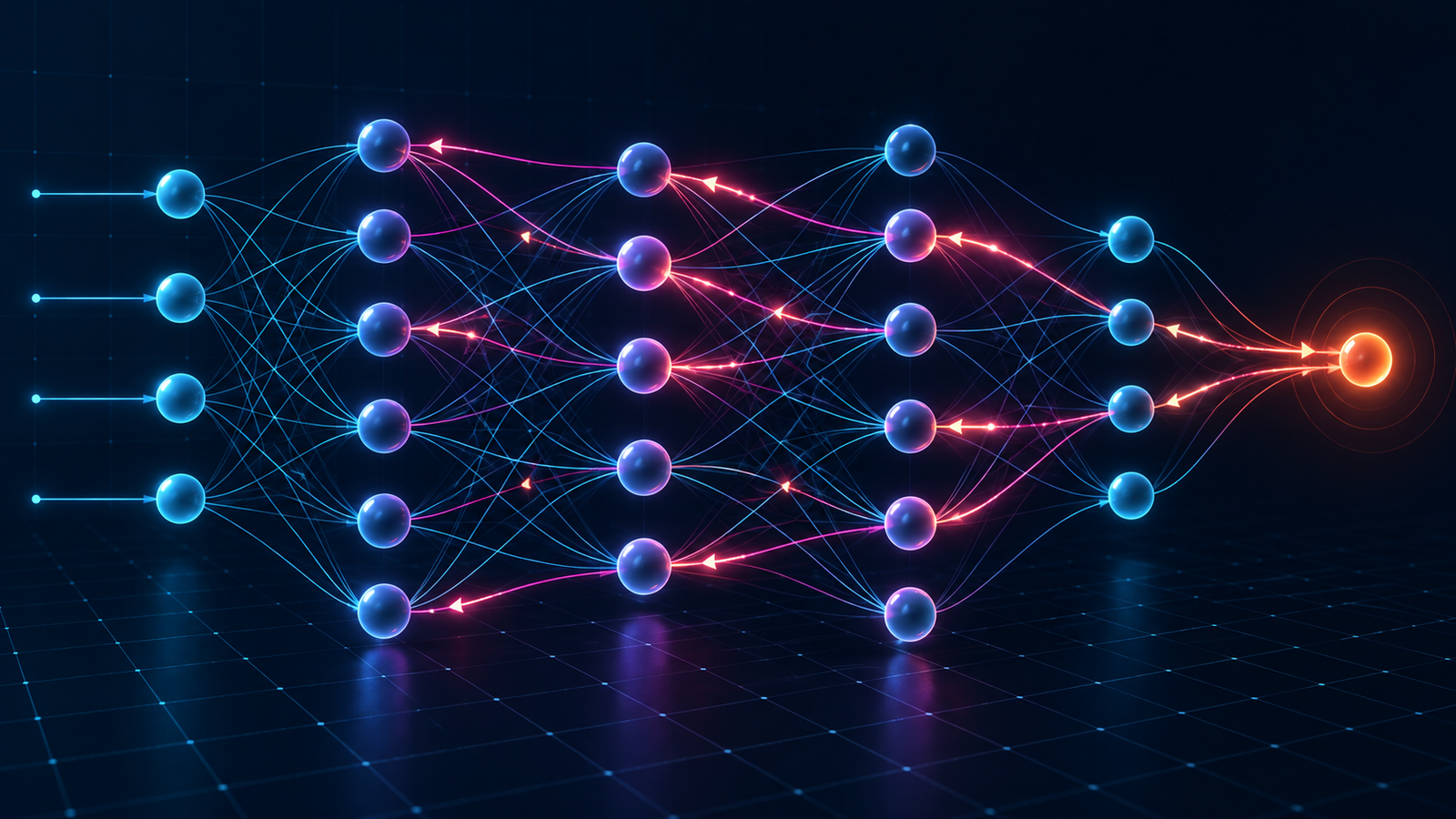
The Model Was Wrong. Which Weight Should We Blame?
A slow, number-by-number journey through backpropagation—from a loss of 0.782 to gradients, updated weights and a better second prediction.
◷ 14 min read
How AI Works
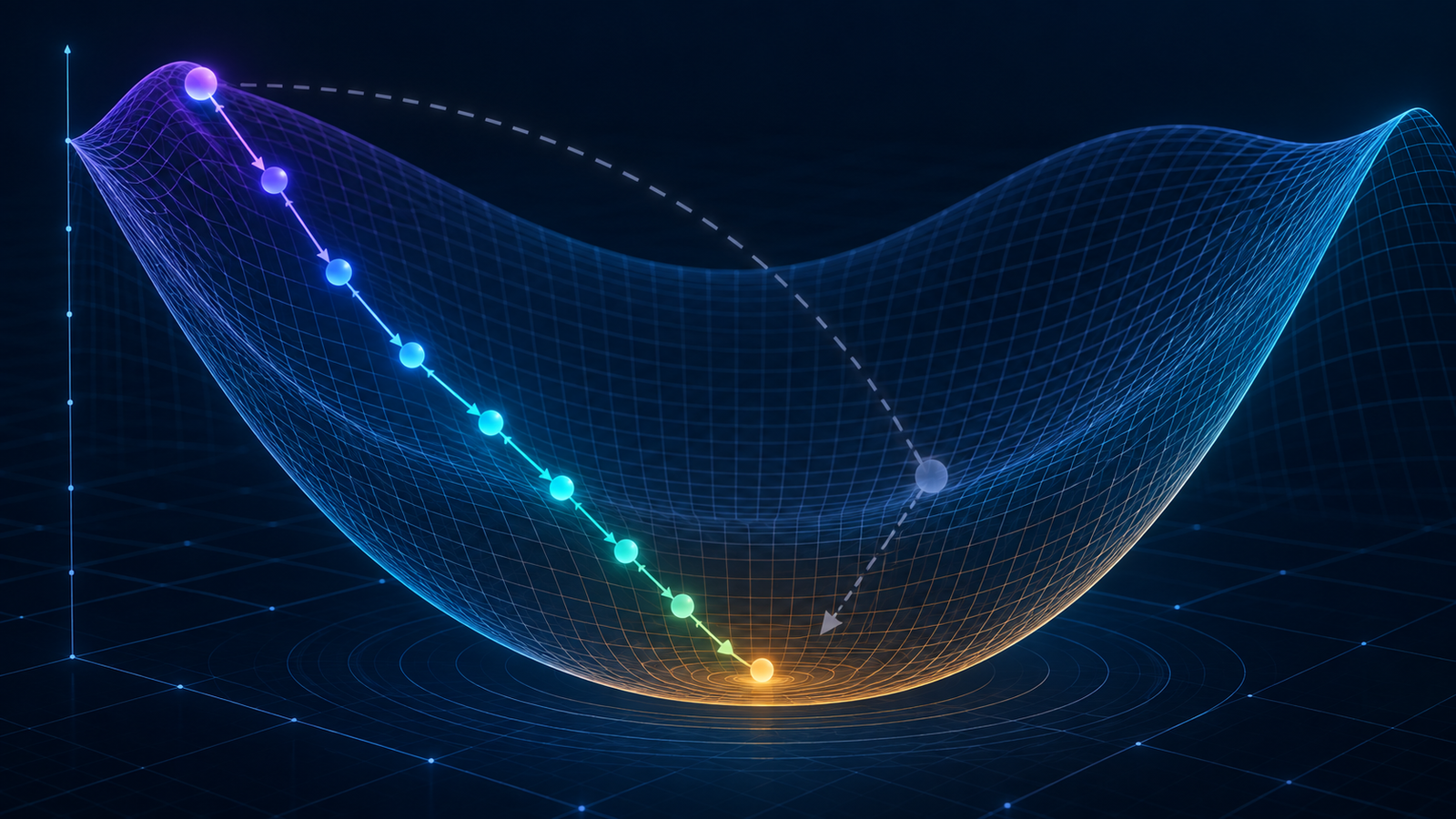
The Gradient Knows the Direction. But How Far Should the Model Move?
A beginner-first explanation of gradient descent, learning rates, loss landscapes, batches, momentum, Adam and AdamW—continuing our neural-network example.
◷ 14 min read

How AI Works
Before a Neural Network Can Learn, It Must Make a Prediction
A slow, number-by-number journey through one forward pass—from ‘The sky is ...’ to a prediction, a probability and a loss.
◷ 15 min read