Mathematics for AI

Why Does AI Need Mathematics?

Here’s a question worth sitting with before we write a single equation:

If you tell a person “make this prediction better,” they understand you instantly. They’ll think about what went wrong, adjust their approach, and try again. No formulas required.

Now try giving that same instruction to a machine.

💡 Think about it “Make this prediction better” means nothing to a computer. A computer doesn’t have judgment. It can only execute precise, mechanical steps — and “better” isn’t a mechanical step. Someone has to translate that vague human intention into something exact enough for silicon to run.

That translation is exactly what mathematics does. It turns a fuzzy human goal into a sequence of computable operations:

"Make this prediction better"
            ↓  (mathematics translates intention into computation)
1. Calculate how wrong the prediction was      →  a LOSS
2. Calculate which direction reduces that error →  a GRADIENT
3. Nudge the internal numbers in that direction  →  an UPDATE
4. Repeat, thousands or millions of times

That is the central training loop, but not the whole engineering story. The result also depends on the data, model design, learning objective, computing system, and evaluation. Mathematics explains the updates; it does not guarantee useful or human-like understanding.

Two words will appear throughout this chapter:

• Training is when a model changes its internal numbers while learning from examples.
• Inference is when a trained model uses those numbers to produce an answer. Its learned numbers normally stay fixed during inference.

For example, showing a model thousands of labeled cat pictures is training. Asking that trained model whether a new picture contains a cat is inference.

🚀 Why This Matters Neural networks, Transformers, and LLMs use the mathematical ideas in this tutorial. You do not need to memorize every formula before continuing. The goal is to recognize what each tool contributes and know where to return for detail.

Here’s the shape of the whole journey, in one line:

REAL WORLD → NUMBERS → VECTORS → MATRICES/TENSORS → FUNCTIONS →
PREDICTION → LOSS → GRADIENT (calculus) → OPTIMIZATION → UPDATED MODEL

Here is the mathematical roadmap for this tutorial:

graph TD
    A[Numbers] --> B[Functions]
    B --> C[Points and Vectors]
    C --> D[Matrices and Tensors]
    D --> E[Probability and Statistics]
    E --> F[Calculus and Gradients]
    F --> G[Optimization]
    G --> H[Attention and Neural Networks]

    style A fill:#f9f,stroke:#333
    style E fill:#bbf,stroke:#333
    style H fill:#bfb,stroke:#333

A Beginner’s Map

You do not need to master every formula in one sitting. The essential path is:

1. Numbers and functions — how a computer represents and transforms information.
2. Vectors and matrices — how many values are organized and processed together.
3. Probability and statistics — how models represent uncertainty and summarize data.
4. Loss, gradients, and optimization — how a model measures mistakes and updates parameters.
5. Attention and LLMs — how the same mathematics is used with language.

Some topics, such as hyperplanes, eigenvectors, and projections, are included as useful previews. They are not required to understand the main training loop on your first read. You can return to them later.

A Few Words You Will See Often

• A number is one value, such as 5.
• A vector is an ordered list of numbers, such as [2, 4, 6].
• A matrix is numbers arranged in rows and columns.
• A tensor is a structured collection of numbers with any number of dimensions.
• A weight is a learned number inside a model.
• Loss is a number that describes how wrong a prediction is.
• A gradient describes how changing a model’s numbers would change its loss.
• Optimization is the process of changing those numbers to reduce the loss.

There is no need to memorize this list yet. We will meet each word again with a small example.

We’re going to walk the chain above one link at a time, starting with the simplest possible question: what does a machine even do with a number?

---

Part 1 — Numbers: The Raw Material of AI

Information processed by a model must be represented numerically. Text can become token IDs and embeddings, images can become pixel values, and audio can become sampled measurements. Choosing a representation matters because different encodings preserve different information.

But not all numbers pull the same weight inside AI. Let’s look at the ones that matter most.

Integers and Decimals

An integer is a whole number — no fractional part: 3, -12, 1000000. In AI, integers show up constantly as counts: number of layers, batch size, number of tokens, vocabulary size.

A decimal (or floating-point number) carries a fractional part: 0.001, 3.14159, -2.7. Almost everything a neural network actually computes with — weights, activations, probabilities — is a decimal, because learning happens through tiny, continuous adjustments, not whole-number jumps.

learning_rate = 0.001      # a decimal — training speed
num_layers = 96            # an integer — a count

Production Reality: Float Precision & Quantization In production AI systems, how we store decimals (floats) affects both speed and memory usage:

• FP32: Uses 32 bits per value and offers more precision than 16-bit formats, at a higher memory and compute cost.
• FP16 and BF16: Use 16 bits per value and are common in modern training and inference. Selected calculations may remain at higher precision for stability.
• INT8 and INT4 quantization: Store or compute selected values with fewer bits. This can reduce memory and sometimes improve speed, but quality and hardware support must be checked.

Negative Numbers

A weight in a neural network can be negative — it means “this input should decrease the output,” not just “contribute less.” Negative numbers give the model a way to express inhibition, not just excitation. Without them, a network could only ever add evidence, never subtract it — and that would make it far too limited to model anything interesting.

Fractions and Ratios

Probabilities live here. For next-token generation, a model can produce a probability distribution over its vocabulary. A value such as 0.83 means the model assigns 83% of its current probability mass to that token under the present context; it does not prove the token is factually correct. After softmax, the values in that distribution add up to 1.

Scientific Notation — Handling Numbers That Don’t Fit on a Page

AI regularly deals with numbers too large or small to write comfortably. A hypothetical model might have 70,000,000,000 parameters, and a gradient update might be 0.000000003. Scientific notation keeps examples like these readable:

70,000,000,000         =  7 × 10¹⁰      (or 7e10)
0.000000003             =  3 × 10⁻⁹     (or 3e-9)

🧠 AI Connection When you see a model described as having “70B parameters,” that “B” is scientific notation in disguise — 7 × 10¹⁰. When you see a learning rate written as 3e-4 in a training script, that’s the exact same idea: 3 × 10⁻⁴, or 0.0003. Once you recognize this pattern, config files stop looking like alphabet soup.

Exponents — The Mathematics of Growth

An exponent means “multiply this by itself, this many times”: 2³ = 2 × 2 × 2 = 8. Exponents show up in AI wherever something grows explosively rather than steadily — the number of possible word combinations in a sentence, the number of parameters as you stack more layers, the compute cost of attention as sequences get longer. Understanding exponents is what lets you understand why scaling a model up isn’t “a bit more expensive” — it’s often dramatically more expensive.

The small raised number is the power. In 2³, the 2 is the base and the 3 says how many times to multiply it. A square is the special case where the power is 2: 5² = 5 × 5 = 25.

Logarithms — The Reverse of Exponents

A logarithm answers the question: “what power do I need to raise this number to, to get that result?” log₂(8) = 3, because 2³ = 8.

Why does AI care? Because probabilities are multiplicative, and multiplication of many small fractions gets numerically painful, fast. Multiply enough probabilities together (each between 0 and 1) and you get numbers so tiny a computer starts losing precision. Logarithms convert that painful multiplication into simple addition:

log(a × b) = log(a) + log(b)

🔊 The Decibels Analogy: Think of logarithms like volume control dials (decibels). Human hearing does not perceive sound intensity linearly; if a sound wave’s power doubles, we do not hear it as twice as loud. Decibels use a logarithmic scale to squash a massive range of sound waves into a clean, human-manageable dial. Similarly, computers use log-probabilities to squash tiny probability fractions into numbers that are easy to add, keeping them from shrinking into silent absolute zero (numerical underflow).

🔍 Under the Hood Log-probabilities and cross-entropy appear frequently in classification and language modeling. Logarithms turn products into sums, preserve ordering because log is increasing, and support numerically stable implementations.

⚠️ Common Mistake Different algorithms use logits, probabilities, log-probabilities, or combinations of them. For example, a stable cross-entropy implementation can work directly from logits. The important lesson is that logarithms make many probability calculations more stable and convenient.

Key takeaway: numbers aren’t just “data” in AI — each type of number (integer, decimal, negative, fraction, huge, tiny) is doing a specific job. Before a machine can learn anything, reality has to be broken down into these raw ingredients.

---

Part 2 — Functions: Turning Inputs Into Outputs

You already understand functions, even if you’ve never thought about them mathematically — you use them every day.

A vending machine is a function: put in B4, get out a bag of chips. A recipe is a function: put in flour, eggs, and sugar, get out a cake. In programming, a function is exactly the same idea:

def double(x):
    return x * 2

double(5)   # → 10

Mathematically, we write this as f(x), read as “f of x” — a rule that takes an input x and produces an output.

    x  ---->  [ FUNCTION f ]  ---->  f(x)
  input                              output

Linear Functions — The Simplest Useful Shape

The simplest interesting function is a straight line:

$$y = mx + b$$

Before using this formula, remember three simple ideas:

• A variable is a name that holds a value, such as x.
• An equation describes a relationship between values.
• A graph gives us a visual way to see that relationship. The horizontal axis usually shows the input, and the vertical axis shows the output.

Here, x is the input, m controls the slope (how steeply the line rises or falls), and b shifts the whole line up or down (the intercept). If m = 2 and b = 1, then f(3) = 2(3) + 1 = 7.

In other words, if x is 3, the equation produces y = 7. The equation is simply a small function that turns an input into an output.

Linear Function Graph:
   y
   |            *
   |         *
   |      *
   |   *
   |*_______________ x

This tiny formula — y = mx + b — might be the single most important shape in this entire tutorial. Hold onto it; it’s about to reappear, barely disguised, as the core operation inside every neural network layer, and again — as a geometric object, not just an algebraic one — in Part 3.

Nonlinear Functions — Adding Bends

Not everything in the world is a straight line. Growth, decisions, and thresholds are usually curved or “bent.” AI relies heavily on two specific nonlinear functions:

ReLU (Rectified Linear Unit) is almost comically simple: if the input is negative, output zero; otherwise, pass it through unchanged.

ReLU(x) = max(0, x)

ReLU(-5) = 0
ReLU(0)  = 0
ReLU(7)  = 7

ReLU Function Graph:
   y
   |       /
   |      /
   |     /
   |    /
___|___/_________ x
   |

Sigmoid squashes any finite input into a value between 0 and 1. That shape is useful for binary probability models, but the output becomes a meaningful probability only when the model, training objective, and evaluation support that interpretation.

        1
sigmoid(x) = -----------
             1 + e^(-x)

sigmoid(-10) ≈ 0.00005   (almost certainly "no")
sigmoid(0)   = 0.5       (completely unsure)
sigmoid(10)  ≈ 0.99995   (almost certainly "yes")

Sigmoid Function Graph:
   y
 1 |         .-----*
   |       ╱
0.5|     *
   |   ╱
 0 | ╱___________ x

🧠 AI Connection These aren’t decorative math trivia — they are functions used inside neural networks to reshape signals. ReLU helps a layer keep useful positive signals, while sigmoid can turn one score into a value between 0 and 1. Without nonlinear functions like these, a neural network — no matter how many layers you stack — would mathematically collapse into a single straight line, incapable of learning anything but the simplest patterns.

The Big Reveal: A Neural Network Is Just a Big Function

Here’s the moment this section has been building toward.

A neural network is not some separate, exotic type of object. It’s a big function, built by chaining many smaller functions together — the output of one becomes the input of the next:

$$F(x) = f_n(\ldots f_2(f_1(x)))$$

   x → [f₁] → [f₂] → [f₃] → ... → [fₙ] → prediction

Each fᵢ is a layer: take the input, apply a linear transformation (y = mx + b, scaled up to thousands of dimensions), then bend it with a nonlinear function like ReLU. Stack enough of these, and the composed function becomes powerful enough to recognize faces, translate languages, or predict the next word in a sentence.

✅ Key takeaway “Neural network” sounds biological and mysterious. Mathematically, it’s just function composition — small, simple functions, layered dozens or hundreds of times, working together to approximate something enormously complicated.

Checkpoint: Before moving on, make sure you can answer:

• What is the input to a function?
• What is the output?
• Why does a neural network use many functions instead of only one?

---

Part 3 — Coordinate Geometry: Giving Numbers a Place

So far, numbers have described quantity — how much of something there is. But an enormous number of real-world questions aren’t about “how much.” They’re about “where.”

For AI, you only need three ideas at first: a point gives data a location, distance tells us how similar two locations are, and dimensions tell us how many measurements describe each item. The sections on lines, planes, and hyperplanes build on this foundation and can be treated as optional detail on a first read.

Points — Pinning Down an Exact Location With Nothing But Numbers

Think about how you’d direct a friend to meet you inside a large office building. You wouldn’t say “somewhere in the building.” You’d say “7th floor, room 12.” Two numbers, and out of possibly thousands of rooms, your friend can walk straight to the exact right one — no guessing required.

That’s the entire idea behind a point. A point answers one question: where is something? In AI, the coordinates can represent measurable features rather than a physical place. For example, a product might be represented by its price and its rating.

We write a 2D point as (x, y):

      y
      |
   4  |        ● (3, 4)
      |
      |________________ x
      0    2

(3, 4) means “3 steps right, 4 steps up.” Nothing about this requires you to be a mathematician — it’s the same idea as a seat number at a cinema, or grid coordinates on a treasure map.

point = (3, 4)                     # a point in 2D space
print("x:", point[0], "y:", point[1])

point_3d = (3, 4, 7)                # one more number → one more dimension
word_point = (0.12, -0.98, 0.44, 0.31, -0.05)   # a "point" in 5D space

🧠 AI Connection When an embedding model represents text with a vector, each number acts as one coordinate in that model’s learned space. The number of coordinates depends on the model. Unlike a room number, one embedding coordinate usually has no simple human-assigned meaning.

Distance — How Far Apart Are Two Things, Exactly?

Once you can name a location, the very next natural question shows up on its own: how far apart are two locations?

Think about how two airports get compared for a flight. Nobody pulls out a physical ruler and a paper map. Instead, each airport has a coordinate (latitude, longitude), and the distance is calculated purely from those numbers — no measuring tape required, ever.

The tool for this is one you likely met in school without realizing how far it would travel: the Pythagorean theorem, repurposed as a distance formula.

The symbol √ means square root. A square root asks: “which number multiplied by itself gives this result?” For example, √25 = 5 because 5 × 5 = 25.

Point A = (1, 1)
Point B = (4, 5)

      y
   5  |        ● B (4,5)
   4  |      ╱ │
   3  |    ╱   │  <- vertical leg = 5 - 1 = 4
   2  |  ╱     │
   1  | ● A(1,1)
      |________│________ x
        1  2  3  4
        horizontal leg = 4 - 1 = 3

distance = √((4-1)² + (5-1)²) = √(9 + 16) = √25 = 5

$$\text{distance} = \sqrt{(x_2-x_1)^2 + (y_2-y_1)^2}$$

Here’s the part that matters enormously for AI: this formula doesn’t care how many dimensions you’re working in. Add a third coordinate, and you just add one more squared term under the square root. Add a thousand, same story.

import math

def distance(p1, p2):
    return math.sqrt(sum((a - b) ** 2 for a, b in zip(p1, p2)))

print(distance((1, 1), (4, 5)))                       # 5.0   — 2D
print(distance((0.1, 0.2, 0.3), (0.4, 0.1, 0.9)))       # works identically in 3D
print(distance((0.1,) * 300, (0.2,) * 300))              # and even in 300D!
# The formula never changes — only the number of terms does.

🧠 AI Connection Euclidean distance is one useful comparison measure. Recommendation, retrieval, and recognition systems may instead use cosine similarity, dot product, learned similarity functions, or domain-specific measures. The correct choice depends on how the vectors were trained and normalized.

⚠️ Common Mistake It’s tempting to think “more dimensions” must eventually make distance calculations unreliable in some exotic way — and there’s a real, named phenomenon here worth knowing: the curse of dimensionality, where in very high-dimensional spaces, most points start to look roughly equidistant from each other, which can make naive distance comparisons less discriminating. This doesn’t mean the formula breaks — it means engineers have to be thoughtful about dimension count, indexing strategy, and which similarity metric they use (more on this in Part 4).

Lines — The Simplest Relationship Between Two Points

A single point answers “where.” Two points immediately raise a new question: what connects them?

Think of a garden hose stretched perfectly taut between two sprinkler heads, with no slack anywhere. Every point along that hose sits in a fixed, predictable relationship to the two ends — that’s the essence of a line: the simplest, most constant possible path connecting two points, extending forever in both directions if you let it.

      y
   5  |        ●
   4  |      ╱
   3  |    ╱
   2  |  ╱
   1  | ●
      |________________ x
        1  2  3  4

You’ve actually already met this idea, from a different angle, in Part 2 — y = mx + b is a line. What’s new here is the lens: instead of thinking of it as “an equation you plug numbers into,” you can now picture it as “a path through space.” Same object, two ways of seeing it.

🧠 AI Connection A concept called linear separability — whether a single straight line (or its higher-dimensional cousin, a hyperplane, coming up next) can cleanly divide two categories of data — is central to classification. Simple models draw exactly this kind of dividing line. The reason deep networks need those nonlinear “bends” from Part 2 is precisely because most real categories in the world aren’t neatly separable by one straight line.

Planes and Hyperplanes — Slicing Through Higher-Dimensional Space

A line lives in flat, 2D space. Step up to 3D, and the natural next shape is a plane — think of an infinite, perfectly flat tabletop, extending in two directions at once, floating at some fixed height in a 3D room.

1D:  a POINT on a line                       ●
2D:  a LINE divides a flat plane             ────────╱────────
3D:  a PLANE divides a cube-shaped space     [ flat sheet slicing through a cube ]
nD:  a HYPERPLANE divides n-dimensional space  [ same idea, impossible to draw ]

A hyperplane is simply “a flat cut through space,” generalized to however many dimensions you need. You can’t draw a hyperplane in 300 dimensions any more than you can picture a 300-dimensional point — but the role it plays never changes: it’s a flat boundary with everything on one side, and everything else on the other.

🧠 AI Connection Support Vector Machines, a classic and still widely used machine learning algorithm, work by finding the best possible hyperplane to separate two categories of data in high-dimensional space. Even inside a modern neural network, each individual neuron’s linear computation (from Part 2) geometrically carves out its own hyperplane in the input space — a network’s real power comes from combining thousands of these simple cuts, bent by nonlinear activations, into wildly complex decision boundaries.

Dimensions — Just a Count, Nothing More

Here’s a reframe that removes almost all of the mystery from this topic. Imagine describing a dish on a restaurant menu using only two numbers: price and calories. That’s a 2D description. Now add spiciness level, prep time, protein content, and a popularity score — you’re now describing that same dish with 7 numbers, which mathematically means: the dish is now a point in 7-dimensional space.

Nothing exotic happened. You simply measured more properties.

1D point:   (5)                                    — one number
2D point:   (5, 3)                                  — two numbers
3D point:   (5, 3, 8)                                — three numbers
7D point:   (5, 3, 8, 1, 9, 2, 4)                     — seven numbers
300D point: (5, 3, 8, 1, ..., 300 numbers total)      — a small word embedding!

🍪 The Cookie Ingredient Analogy: Think of dimensions as different measurements of a cookie:

• 1D (Sweetness): A sweet onion biscuit and a chocolate chip cookie might sit near each other because they are both sweet.
• 2D (Sweetness + Saltiness): They begin to separate.
• 3D (Sweetness + Saltiness + Crunchiness): They are now clearly in separate locations.
• 100D: More coordinates can record more aspects of the cookie, but they do not identify it perfectly. The measurements must be useful, the data must be good, and irrelevant dimensions can add noise.

point_2d = (3, 4)
point_7d = (3, 4, 1, 9, 0, 2, 6)
point_300d = tuple(range(300))

print(len(point_2d))    # 2   — "this point lives in 2D space"
print(len(point_7d))    # 7   — "this point lives in 7D space"
print(len(point_300d))  # 300 — "this point lives in 300D space"

A patient’s record may contain height, blood pressure, heart rate, age, and many lab values. Mathematically, that record can be represented as a point with many coordinates. A clinician uses far more context and judgment than this vector alone; the example only explains numerical representation.

🔍 Under the Hood Human vision evolved to navigate a 3D physical world, which is exactly why we can picture points, lines, and planes up through 3 dimensions — and hit a wall immediately after. The good news: the algebra itself never notices this limitation. Computing the distance between two 300-dimensional points uses the identical formula as computing distance in 2D — just with 300 terms instead of 2.

High-Dimensional Spaces — Where AI Actually Lives

Try describing the word “king” using only two numbers. You’d be forced to throw away almost everything that makes “king” meaningfully different from “queen,” “president,” or “chess piece.” There simply isn’t enough room in two numbers to hold all of that nuance.

Now imagine many more coordinates. The model has more capacity to arrange useful relationships, but one coordinate does not normally equal one named idea such as “royalty.” Information is usually distributed across many coordinates working together.

1D:    king ●───────● queen        (barely distinguishable — everything is crammed onto one line)

2D:    king ●
              ╲                     (a little more room — maybe one axis for
               ● queen                "royalty" and another for "gender")

high-D: each item receives coordinates in one model's learned space.
        The coordinates work together and are not independent,
        human-labeled "axes of meaning."

Real embedding models use different dimension counts. OpenAI documents text-embedding-3-large with 3,072 dimensions by default and supports shortening its output. Open models also use varied sizes. Dimension count alone does not reveal which model retrieves better.

A production semantic-search system embeds a query, searches an index using the metric expected by that model, and may apply metadata filters or reranking. Approximate indexes trade a small amount of recall for much faster search at scale.

⚠️ Common Mistake Beginners often assume “more dimensions is automatically better.” In practice, embedding size is a deliberate engineering trade-off: more dimensions can capture richer meaning, but they also cost more memory and more computation per comparison, and can run into the curse of dimensionality mentioned earlier. Bigger isn’t free, and it isn’t always better — which is exactly why techniques exist specifically to shrink these spaces back down when needed, while trying to preserve their most important relationships.

✅ Key takeaway Everything in this section boils down to one reassuring fact: the mathematics of points, distance, lines, and planes never changes as dimension count grows. Only the number of terms in each formula grows. You don’t need to visualize 1,536 dimensions to trust the arithmetic — you just need to trust that the same simple rules from 2D keep working, over and over, no matter how large the space gets. That trust is exactly what lets AI comfortably operate in spaces no human will ever be able to picture.

Reading tip: The most important parts of this section are points, distance, and dimensions. Hyperplanes and high-dimensional geometry are useful previews, but you can return to their details after you understand vectors and embeddings.

---

Part 4 — Vectors: Numbers With Direction

A plain number tells you how much. A vector tells you how much, in which direction.

Here’s the distinction, made concrete. Saying “walk 500 meters” gives you a magnitude but no direction — you have no idea which way to go. Saying “walk 500 meters northeast” gives you both. Every turn-by-turn direction you’ve ever followed from a maps app was secretly a sequence of vectors the whole time.

number:  "5 kilometers"
vector:  "5 kilometers, heading northeast"

We write a vector as a list of numbers, like v = [2, 3] — and instead of reading it as “a location,” we now read it as an arrow, starting at the origin and pointing toward (2, 3).

  y
  |
3 |        ↗
  |      ↗
  |    ↗
  |  ↗
  |________________ x
  0    2

See the parts of a vector together

The diagram below uses v = [3, 4]. Read the two numbers as instructions: move 3 units along the x-axis, then 4 units along the y-axis. Together, those components create one arrow from (0, 0) to (3, 4).

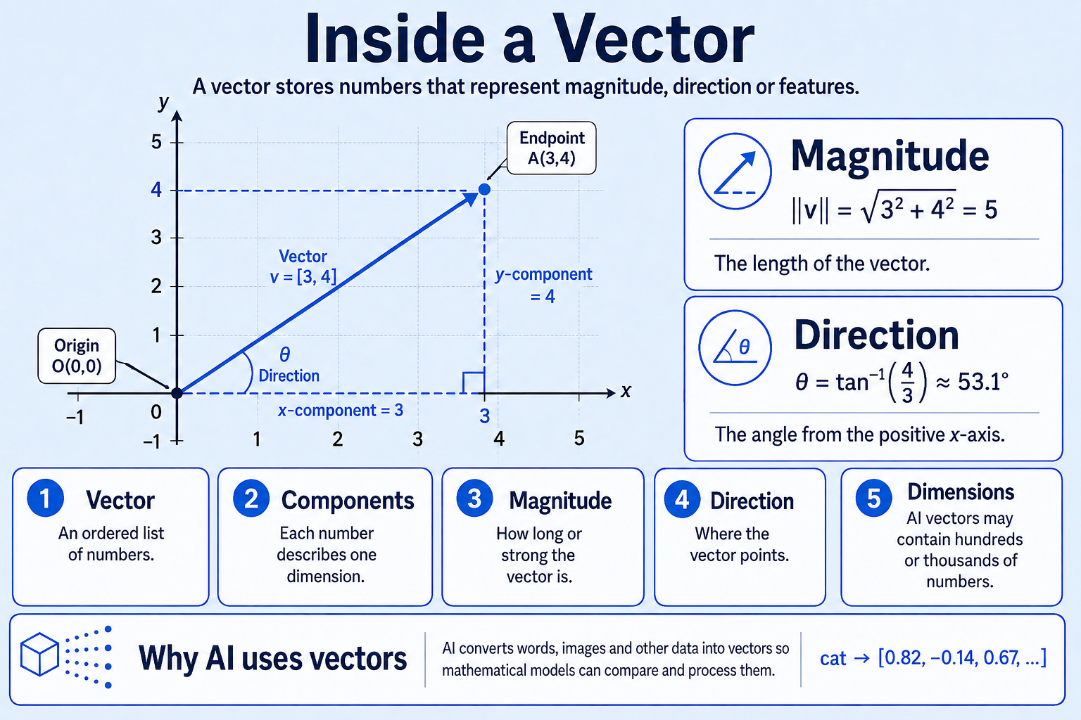
How the 2D picture connects to AI

• In two dimensions, [3, 4] is easy to draw because it has only an x-component and a y-component.
• Its magnitude is √(3² + 4²) = 5, so the arrow is 5 units long.
• Its angle is about 53.1° from the positive x-axis. The diagram’s tan⁻¹(4/3) calculation works for this first-quadrant example; software commonly uses atan2(y, x) because it also handles other quadrants and zero x-values correctly.
• An AI embedding may contain hundreds or thousands of components. We cannot draw all those dimensions, but the same rules for components, magnitude, distance, and similarity still apply.
• An embedding’s direction is not a physical compass direction. It describes a mathematical relationship in a space learned by the model, where vectors pointing in similar directions may represent related information.

[3, 4]
  │  │
  │  └── 4 units along y
  └───── 3 units along x
       ↓
one vector with magnitude 5 and direction 53.1°

💡 Think about it A point tells us where something is. A vector tells us how far and in which direction to move. They can use the same coordinates, but they answer different questions:

Point:  (3, 4) means "the object is here"
Vector: (3, 4) means "move 3 steps right and 4 steps up"

In AI, we often use the same list of numbers in both ways: as a location in a representation space or as a direction and magnitude for a calculation.

Direction — Which Way an Arrow Points, Independent of Its Length

A compass needle points north whether it’s a tiny needle on a cheap keychain or a large one mounted on a ship’s deck — its size doesn’t change what direction it indicates. Vectors work the same way: two vectors can point in exactly the same direction while having very different lengths.

      y
   8  |  ● (6, 8)   <- vector A, LONG
   4  |  ● (3, 4)   <- vector B, SHORT
      |╱ ╱
      |________________ x
        3    6

Vector A = (6, 8) and Vector B = (3, 4) point in exactly the same direction — A is simply twice as long. In meaning-space, this pattern shows up constantly: it often represents “the same underlying idea, expressed with different intensity.”

Magnitude — How Long Is the Arrow?

Magnitude (also called the norm) measures a vector’s length — its “how much,” stripped of direction. Wind isn’t just “blowing northeast” — it’s “blowing northeast at 40 km/h.” A weather app that reported only direction, never speed, would be nearly useless. Magnitude is what fills in the “how much” half of the picture.

Convenly, magnitude uses the exact same formula as distance from Part 3 — just measured from the origin instead of between two arbitrary points:

$$\|v\| = \sqrt{v_1^2 + v_2^2 + \ldots}$$

For v = [3, 4]: magnitude = √(3² + 4²) = √25 = 5.

import numpy as np

v = np.array([3, 4])
print(np.linalg.norm(v))   # 5.0

embedding = np.array([0.12, -0.98, 0.44, 0.31])
print(np.linalg.norm(embedding))   # the "length" of a real embedding vector

🧠 AI Connection Magnitude shows up constantly in AI engineering: gradient magnitude is monitored during training to catch a model whose updates are growing unstable (exploding gradients) or shrinking toward zero (vanishing gradients — discussed in Part 8). L2 regularization discourages large parameter magnitudes, although the effect on generalization depends on the model and training setup.

Unit Vectors — Keeping Only the Direction

Sometimes you want just the direction from a vector, with the length completely removed — set to exactly 1. That’s a unit vector: it points the same way as the original, but its magnitude is forced to be exactly one.

Think of it as trading a ruler-and-arrow for a plain compass: all that survives is “which way,” nothing about “how far.”

v = (3, 4), magnitude = 5

unit vector = v / magnitude = (3/5, 4/5) = (0.6, 0.8)

Check: magnitude of (0.6, 0.8) = √(0.6² + 0.8²) = √(0.36 + 0.64) = √1 = 1 ✓

v = np.array([3, 4])
unit_v = v / np.linalg.norm(v)
print("unit vector:", unit_v)          # [0.6, 0.8]
print("its magnitude:", np.linalg.norm(unit_v))   # 1.0, always, by construction

🧠 AI Connection Many embedding models deliberately normalize their output vectors into unit vectors before storing them — precisely so that later similarity comparisons depend purely on meaning (direction), and aren’t quietly skewed by incidental factors like how long a piece of text happened to be.

Distance, Revisited Through Vectors

You already learned the distance formula in Part 3. Vectors give you a cleaner way to say the same thing: the distance between two points is simply the magnitude of the vector that connects them.

Point A = (1, 1)      Point B = (4, 5)

difference vector = B - A = (4-1, 5-1) = (3, 4)
distance(A, B) = magnitude of (3, 4) = √(9 + 16) = 5

A = np.array([1, 1])
B = np.array([4, 5])
diff = B - A
print("difference vector:", diff)         # [3 4]
print("distance:", np.linalg.norm(diff))   # 5.0 — same answer as Part 3

Nothing new was invented here — it’s the same formula from Part 3, just reframed through the lens of “how far, and in which direction, is B from A.”

The Dot Product — Measuring How Aligned Two Vectors Are

The dot product multiplies two vectors’ matching components and adds up the results:

$$v \cdot w = v_1 w_1 + v_2 w_2 + \ldots$$

See what the dot product measures

The diagram uses a = [3, 0] and b = [2, 2]. Vector a points directly along the positive x-axis, while vector b points upward at a 45° angle. The dot product measures how much the vectors point together, while also including their lengths.

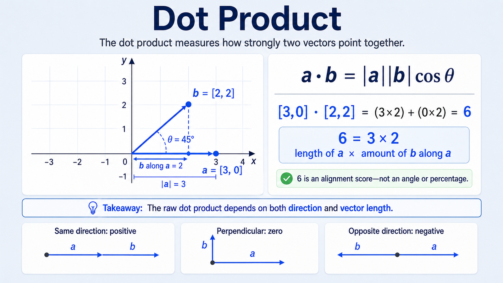
Read the calculation in two connected ways

Matching components:             Geometric view:

[3, 0] · [2, 2]                  length of a = 3
= (3 × 2) + (0 × 2)              amount of b along a = 2
= 6 + 0                          3 × 2
= 6                              = 6

• The first method multiplies matching components and adds the results.
• The second method asks how much of b lies in a’s direction, then multiplies that amount by the length of a.
• A positive result means the angle is less than 90°; zero means the vectors are perpendicular; a negative result means they point more against each other than together.
• The raw result 6 is neither an angle nor a percentage. Making either vector longer can increase the dot product even when the angle stays unchanged.
• If you normalize both vectors to length 1, their dot product becomes cosine similarity. That normalized score isolates direction by removing the effect of vector length.

v = np.array([2, 3])
w = np.array([4, 5])
np.dot(v, w)   # → 2*4 + 3*5 = 8 + 15 = 23

The dot product combines direction and magnitude. A positive value indicates an angle below 90 degrees, zero indicates perpendicular vectors, and a negative value indicates an angle above 90 degrees. A large value can result from stronger alignment, larger magnitudes, or both.

Cosine Similarity — A Common Direction-Based Comparison

Here’s a scenario worth sitting with. Two product reviews can say almost exactly the same thing even if one is a short sentence and the other is several paragraphs. Their embeddings may point in a similar direction. Their lengths may still differ for several reasons, so comparing only raw distance could make them look less similar than they are.

If you compared these two vectors using plain Euclidean distance from Part 3, the length difference alone could make them look far apart — even though they’re saying the same thing. That’s the exact gap cosine similarity was built to close: a way to compare vectors purely by the angle between them, with magnitude completely divided out.

💡 Think about it Imagine two speakers playing the exact same song — one quietly, one at full volume. Judging “are these the same song?” by loudness alone would be a bad approach. You’d listen to the pattern, not the volume. Cosine similarity does the mathematical equivalent: it compares the “pattern” (direction) and deliberately ignores the “volume” (magnitude).

The formula divides the dot product by the product of both vectors’ magnitudes, which cancels out length entirely:

$$\cos(\theta) = \frac{v \cdot w}{\|v\| \, \|w\|}$$

See cosine similarity ignore length

The diagram compares A = [2, 2], B = [4, 4], and C = [-2, 2]. Vector B is twice as long as A, but both point in exactly the same direction. Cosine similarity therefore gives them the maximum directional score of 1.

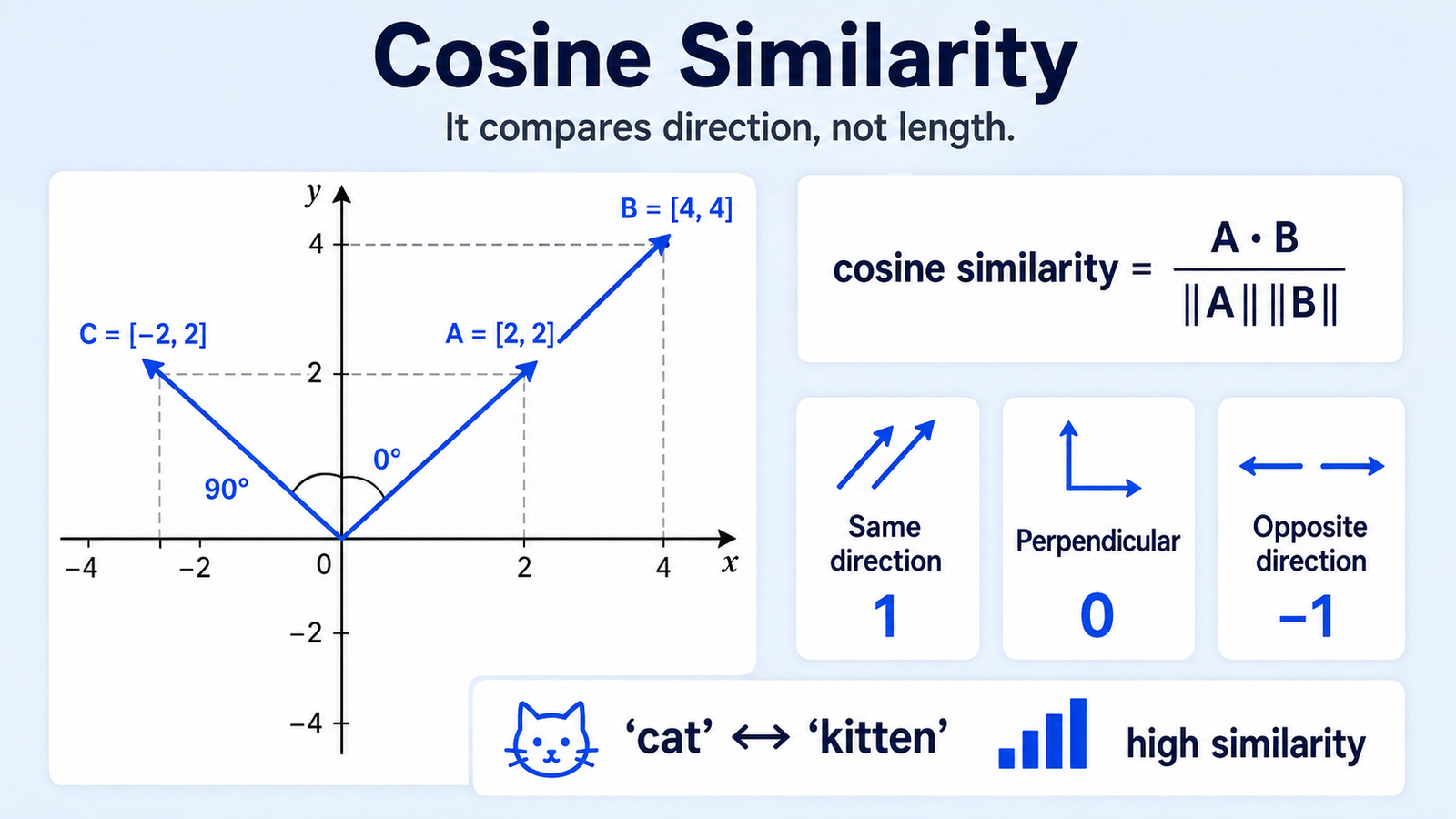
Follow the angles in the picture

• A and B have a 0° angle, so their cosine similarity is 1. Their different lengths do not change that score.
• A and C have a 90° angle, so their cosine similarity is 0. In this geometric example, they have no directional alignment.
• Two vectors pointing in exactly opposite directions have a 180° angle and cosine similarity -1.
• Vector B is drawn with its tail shifted to keep the graphic readable. A vector can be moved without changing its components; imagine both A and B beginning at the origin when comparing their directions.
• The cat ↔ kitten example is an intuition, not a universal promise. Whether two word embeddings have high cosine similarity depends on the embedding model and how it was trained.

same direction       → cosine =  1
right angle          → cosine =  0
opposite direction   → cosine = -1

Here is how cosine similarity compares vectors purely by angle, regardless of how long they are:

graph TD
    O(Origin) -->|Vector A: Short| V1["'Cat' (Word)"]
    O -->|Vector B: Long| V2["'Feline' (Paragraph)"]
    O -->|Vector C: Perpendicular| V3["'Banana' (Word)"]

    style V1 fill:#dfd,stroke:#333
    style V2 fill:#dfd,stroke:#333
    style V3 fill:#fdd,stroke:#333

In this diagram, Vector A and Vector B point in a similar direction (high cosine similarity = ~1.0) despite being very different lengths. Vector C points in a perpendicular direction (cosine similarity = ~0.0), representing an unrelated concept.

A worked example. Let v = (1, 2) and w = (2, 4) — notice w is exactly 2×v, same direction, different length.

dot product = (1×2) + (2×4) = 2 + 8 = 10
magnitude of v = √5
magnitude of w = √20

cosine similarity = 10 / (√5 × √20) = 10 / 10 = 1.0

A perfect score of 1.0, correctly recognizing that v and w point in identical directions, despite w being twice as long.

def cosine_similarity(v, w):
    dot_product = np.dot(v, w)
    return dot_product / (np.linalg.norm(v) * np.linalg.norm(w))

v = np.array([1, 2])
w = np.array([2, 4])    # same direction, 2x magnitude
u = np.array([2, -1])   # a very different direction

print(cosine_similarity(v, w))   # 1.0  — identical direction
print(cosine_similarity(v, u))   # close to 0 — unrelated direction

For nonzero vectors, the result lies between -1 and 1: 1 means identical direction, 0 means perpendicular, and -1 means opposite direction. Whether those values mean “similar” or “unrelated” depends on how the embedding model was trained. Cosine similarity is undefined for a zero vector.

| Score | Meaning                         |
|-------|----------------------------------|
| 1.0   | Identical direction (max similar) |
| 0.0   | Perpendicular — unrelated         |
| -1.0  | Opposite direction                |

Production Reality: Vector Database Normalization Some embedding pipelines normalize vectors before indexing. For unit vectors, cosine similarity equals the dot product. Other systems use dot product or Euclidean distance directly. Follow the embedding model and vector-index documentation rather than normalizing automatically.

Embeddings, Properly Introduced

An embedding is a learned vector representation of an item such as text, an image, or a product. Useful relationships can appear as geometric relationships in the learned space. Meaning is distributed across the vector and is not always represented only by direction.

"king"   → [0.21, -0.45, 0.88, ...]
"queen"  → [0.19, -0.40, 0.91, ...]
"banana" → [-0.72, 0.11, -0.05, ...]

⚠️ Common Mistake It’s tempting to imagine embeddings “contain” dictionary definitions somewhere inside those numbers. They don’t. A model learns these numerical positions purely so that useful relationships — similar words landing near each other, related concepts pointing in similar directions — fall out of training. Nobody hand-designs what any individual number means, and there’s no guarantee two different embedding models place “king” and “queen” anywhere near the same coordinates as each other.

Depending on its training, an embedding model may place “king” and “queen” closer than “king” and “banana.” Semantic search compares query and stored embeddings, often using cosine similarity or dot product. A production RAG retriever may also use keyword search, access filters, approximate indexing, and reranking.

🚀 Why This Matters Embedding similarity often helps retrieval systems find relevant context for a chatbot. The language model itself uses learned representations and attention internally; it does not answer every prompt by running a vector-database cosine search.

Checkpoint: Before moving on, make sure you can answer:

• What does a vector represent?
• What does its magnitude tell us?
• What does cosine similarity compare?

---

Part 5 — Matrices: Processing Many Relationships at Once

A vector is great for representing one thing. But a real neural network layer might take in 768 numbers and need to produce 768 new numbers — and it needs to do this for millions of examples, fast. You wouldn’t want to write 768 separate y = mx + b equations by hand. You need a way to describe many linear transformations at once.

That’s a matrix — a grid of numbers, organized into rows and columns.

W = [[1, 2],
     [3, 4],
     [5, 6]]

This matrix has shape (3, 2) — 3 rows, 2 columns. Shape is one of the most important ideas in this entire tutorial; almost every practical deep-learning bug traces back to a shape mismatch somewhere.

Matrix Operations

Addition works element by element, same as vectors — and requires matching shapes.

Transpose flips a matrix over its diagonal, turning rows into columns:

       [[1, 2],            [[1, 3, 5],
W  =   [3, 4],    Wᵀ  =     [2, 4, 6]]
       [5, 6]]

Matrix multiplication is where the real power lives. To multiply matrix A by matrix B, you take the dot product of each row of A with each column of B — the exact dot product you just met in Part 4, applied many times at once.

You can think of matrix multiplication as a fast way to apply many related calculations together. Each row of the first matrix describes one calculation, and each column of the second matrix supplies the values that calculation uses.

When multiplying two matrices, the shapes must align. You can visualize this dimension-matching rule like this:

graph TD
    A["Matrix A: shape (3 x 2)"] -->|Columns of A must equal...| C["Match: 2"]
    B["Matrix B: shape (2 x 4)"] -->|...Rows of B| C
    C --> Result["Result Matrix: shape (3 x 4)"]

The number of columns in A must equal the number of rows in B.

A = np.array([[1, 2],
              [3, 4]])
B = np.array([[5, 6],
              [7, 8]])
A @ B
# → [[1*5+2*7, 1*6+2*8],
#    [3*5+4*7, 3*6+4*8]]
# → [[19, 22],
#    [43, 50]]

An identity matrix is the matrix equivalent of multiplying by 1 — it leaves anything it multiplies unchanged. A matrix inverse is a special matrix that can undo a transformation when an inverse exists. It is somewhat similar to division, but not every matrix can be inverted. You won’t need to compute inverses by hand in AI work; the useful intuition is simply that some transformations can be reversed and some cannot.

A Core Equation Inside Many Neural Network Layers

Remember y = mx + b from Part 2? Scale it up from single numbers to entire vectors and matrices, and you get:

$$y = Wx + b$$

• x — the input vector (e.g., an embedding)
• W — a matrix of learned weights
• b — a vector of learned biases
• y — the output vector, ready for the next layer

A tiny worked example. Suppose x = [1, 2], W = [[2, 0], [1, 1]], b = [0, 1]:

Wx = [[2, 0],   [1]   [2*1 + 0*2]   [2]
      [1, 1]] × [2] = [1*1 + 1*2] = [3]

y = Wx + b = [2, 3] + [0, 1] = [2, 4]

🧠 AI Connection y = Wx + b is the affine part of many neural-network layers. An activation or another operation often follows it. Architectures can also contain normalization, attention, convolutions, routing, and residual connections. Learned parameters include weights, biases, and sometimes other adjustable values.

🔍 Under the Hood GPUs were developed for parallel graphics workloads, but the same parallel hardware is well suited to large matrix operations. Modern AI accelerators also optimize data movement, reduced-precision arithmetic, and specialized tensor operations.

---

Part 6 — Tensors: When Two Dimensions Aren’t Enough

Let’s line up what we’ve built so far:

Object	Dimensions	Example
Scalar	0D	7
Vector	1D	[2, 3, 5]
Matrix	2D	[[1, 2], [3, 4]]
Tensor	nD	scalar, vector, matrix, or higher-rank array

In deep-learning software, a tensor is a multidimensional array of numbers with a data type, shape, and device. A scalar is rank 0, a vector rank 1, and a matrix rank 2. People often start saying “tensor” when rank reaches 3, but the lower-rank objects are tensors too. This software definition is enough here; tensors have a deeper mathematical definition in advanced mathematics.

Why would you ever need that many? Because real-world data isn’t flat.

A single color image:    (height, width, channels)
A batch of images:       (batch, height, width, channels)
A video:                 (batch, time, height, width, channels)

🧵 The Fabric Stack Analogy:

• Scalar (0D): A single bead.
• Vector (1D): A string of beads.
• Matrix (2D): A flat sheet of fabric woven from strings.
• Tensor (3D): A stack of fabric sheets (forming a block of cloth).
• Tensor (4D): A warehouse containing a row of stacks of fabric.

A 224×224 color photo might use shape (224, 224, 3): height, width, channels. A batch of 32 then has shape (32, 224, 224, 3). Some frameworks or models instead put channels first, producing (32, 3, 224, 224). A shape is meaningful only when you also know what each axis represents.

import numpy as np
batch = np.zeros((32, 224, 224, 3))
batch.shape   # → (32, 224, 224, 3)

⚠️ Common Mistake Shape mismatches are a common source of deep-learning bugs. “Expected shape (32, 128) but got (128, 32)” means the same numbers were organized along different axes. Write down axis names—not just sizes—when debugging.

🧠 AI Connection This is exactly why frameworks like PyTorch and TensorFlow are built entirely around tensor objects, not plain arrays — they need efficient, GPU-friendly containers for these multi-dimensional blocks of numbers, whether that’s a batch of images, a batch of audio clips, or a batch of token sequences flowing through an LLM.

---

Part 7 — Probability and Statistics: Reasoning Under Uncertainty

AI rarely receives perfect information. A photo may be blurry, two words may fit the same sentence, and tomorrow’s sales are not known yet. Probability gives a model a language for uncertainty; statistics helps us learn from and evaluate collections of observations.

Probability Is a Number Between 0 and 1

A probability of 0 means an event is treated as impossible under the model. A probability of 1 means it is treated as certain. Values in between describe uncertainty.

Suppose a model assigns these probabilities to the next token after “The sky is”:

Token	Probability
blue	0.60
clear	0.25
dark	0.10
other tokens combined	0.05

The values add to 1.00. The model may select the largest value, or a sampling method may sometimes choose another plausible token. These are model probabilities, not guarantees about the real world.

See a probability distribution

The diagram below shows the model sharing all available probability across four possible next tokens. A taller bar means the model considers that token more likely in the current context; it does not mean that token is guaranteed to be correct or selected.

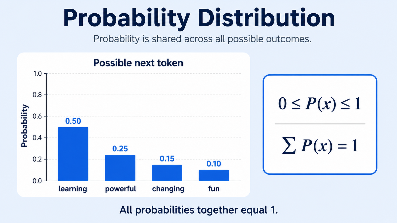
Read the numbers step by step

learning  = 0.50
powerful  = 0.25
changing  = 0.15
fun       = 0.10
           ────
total     = 1.00

• 0.50 means the model assigns 50% of its probability mass to learning among the outcomes shown.
• No probability is below 0 or above 1.
• The complete set adds to 1, which is the same as 100%.
• This is a simplified four-token example. A real language model usually spreads probability across a vocabulary containing many thousands of possible tokens, including choices with extremely small probabilities.
• These values depend on the preceding text. Change the prompt or earlier tokens, and the entire distribution can change.

Mean, Median, and Variance

Suppose five request times are:

100 ms, 110 ms, 120 ms, 130 ms, 540 ms

• The mean is the total divided by the count: (100 + 110 + 120 + 130 + 540) / 5 = 200 ms.
• The median is the middle value after sorting: 120 ms.
• Variance measures how spread out values are around the mean. Its square root is the standard deviation, expressed in the original unit.

The slow 540 ms request pulls the mean upward, while the median remains closer to a typical request. AI teams use summaries like these to understand data distributions, loss values, latency, and evaluation scores.

Why this matters

An average can hide important groups. A speech model might have 95% average accuracy while performing much worse for one accent. Always inspect the distribution and meaningful subgroups, not only one headline number.

Conditional Probability

Conditional probability asks: What is the probability of A when we already know B?

For example, “What is the chance an email is spam?” is different from “What is the chance it is spam given that it contains an unfamiliar payment link?” We write this as:

$$P(A \mid B)$$

The vertical bar means “given.” Models repeatedly make predictions conditioned on available input. A language model estimates possible next tokens given the tokens already in its context.

Bayes’ Rule: Update a Belief With Evidence

Imagine that only 1 in 100 school emails is truly malicious. A detector catches most malicious emails, but it also raises some false alarms. When the detector warns you, the original rarity still matters: a warning does not automatically mean the email is malicious.

Bayes’ rule combines:

• the starting frequency, called the prior;
• how likely the evidence is under each possibility; and
• the updated probability after seeing evidence, called the posterior.

This is why medical tests, fraud detectors, and spam filters must be evaluated with real event frequencies. A highly accurate detector can still create many false alarms when the event is rare.

A worked example with 1,000 emails:

10 are malicious.
The detector correctly flags 9 of those 10.

990 are safe.
If it falsely flags about 5% of safe emails, that is about 50 false alarms.

Total warnings ≈ 9 true warnings + 50 false warnings = 59
Chance a warned email is truly malicious ≈ 9 / 59 ≈ 15%

The detector caught 90% of malicious emails, yet most warnings were false because malicious email was rare. This is the base-rate effect.

From Scores to a Probability Distribution

A neural network often produces raw scores called logits. Softmax converts a group of logits into positive values that add to 1.

logits:        [2.0, 1.0, 0.1]
                  ↓ softmax
probabilities: [0.66, 0.24, 0.10]   (rounded)

Softmax preserves order—the largest logit receives the largest probability—but the gaps and temperature affect how concentrated the distribution becomes.

Cross-Entropy Connects Probability to Loss

If the correct class is “cat,” training should reward a high probability for “cat” and penalize a low one. A simplified loss for the correct class is:

$$L = -\log(p_{\text{correct}})$$

Probability assigned to correct class	Approximate loss
0.90	0.105
0.50	0.693
0.10	2.303

Confidently assigning the correct answer a low probability produces a large penalty. This gives calculus and optimization a single number to reduce.

Checkpoint: You should now be able to explain why probabilities add to one in a softmax distribution, why an average can hide outliers, what “given” means in conditional probability, and how cross-entropy rewards probability placed on the target.

---

Part 8 — Calculus: How Does AI Know How to Improve?

Here’s where the story turns a corner. Everything so far has been about representing information — numbers, vectors, matrices, tensors. Now we ask a completely different question:

A model just made a bad prediction. How does it know which of its millions of internal numbers to change, and in which direction?

The Hiking Trail Intuition

Imagine you’re standing on a foggy mountainside, blindfolded, and you’re told: “get to the lowest point.” You can’t see the whole landscape. But you can feel the ground tilting under your feet, right where you’re standing.

💡 Think about it If the ground slopes down to your left, you step left. That’s it — you don’t need a map of the entire mountain. You just need to know the slope under your current position, and you can take one good step at a time.

That local slope is exactly what a derivative measures.

Derivatives — Slope at a Single Point

For a simple function like f(x) = x², the derivative tells you how steeply the function is rising or falling at any given point x:

f(x) = x²
f'(x) = 2x     (the derivative)

At x = 3:  slope = 2(3) = 6   → rising steeply
At x = 0:  slope = 2(0) = 0   → flat, the bottom of the curve
At x = -3: slope = 2(-3) = -6 → falling steeply

   f(x)
    |    *                *
    |     *              *
    |      *            *
    |       *          *
    |        *        *
    |         *______*
    |          (x=0, minimum)
    |________________________ x

Notice something important: at x = 0, the slope is exactly zero — and for this bowl-shaped curve, that is the point with the lowest value. In general, a zero slope can indicate a minimum, maximum, or flat point. This gives us the intuition for Part 9: slopes help us search for useful low points in a loss function.

Partial Derivatives and Gradients

A real neural network doesn’t have one variable — it has millions or billions of them (every weight in every W matrix). A partial derivative asks: “if I nudge just this one weight, and hold everything else fixed, how does the output change?”

🎛️ The Drone Control Board Analogy: Imagine piloting a drone in thick fog, trying to find a landing pad. You can’t see the ground, but you have a console with 1,000 knobs (representing 1,000 model weights):

• Partial Derivative: You turn Knob 1 slightly; you feel the drone tilt 2 inches North. You turn Knob 2 slightly; the drone tilts 1 inch South. You calculate this effect for each of the 1,000 knobs individually.
• Gradient: The master vector that combines all 1,000 individual knob adjustments. It points in the direction that will cause the drone to climb fastest (uphill).
• Optimization: Since you want to land, you move in the opposite direction (negative gradient), adjusting all 1,000 knobs simultaneously to descend toward the ground (minimum loss).

Collect the partial derivatives of a scalar loss with respect to the trainable parameters, and you get the gradient. Under the usual Euclidean geometry, it points toward the steepest local increase. Its negative points toward the steepest local decrease.

gradient = [ ∂L/∂w₁, ∂L/∂w₂, ∂L/∂w₃, ... ]

🚀 Why This Matters The gradient is the mathematical answer to “which direction goes uphill, across millions of dimensions at once.” Reverse its direction, and you know exactly which way is downhill — which is precisely what a model needs to reduce its error.

The Chain Rule and Backpropagation

Remember from Part 2 that a neural network is a composition of functions: F(x) = fₙ(...f₂(f₁(x))). To find how the final error depends on a weight buried deep inside an early layer, you need to trace the effect of that weight through every single function it passes through on the way to the output.

The chain rule is the mathematical tool that makes this tractable: it lets you compute the derivative of a composed function by multiplying the derivatives of each individual step.

Backpropagation efficiently applies the chain rule backward through a recorded computation graph. It computes gradients for trainable parameters that influenced the loss. The optimizer then decides how to use those gradients; backpropagation itself does not update the weights.

INPUT → layer 1 → layer 2 → ... → layer n → PREDICTION → ERROR
                                                               |
        ←──────────── gradients flow backward ───────────────┘
        (chain rule computes each layer's contribution to the error)

🔍 Under the Hood When PyTorch calls .backward() on a scalar loss, autograd follows recorded differentiable operations and accumulates gradients for connected tensors that require them. Detached, frozen, nondifferentiable, or unused values do not automatically receive useful gradients.

Key takeaway: calculus doesn’t make the model smart. It gives the model a precise, computable answer to one question — “which direction reduces my error?” — for every single one of its parameters, simultaneously.

Checkpoint: Before moving on, make sure you can answer:

• What does a derivative measure?
• What does a gradient tell the model?
• Why does gradient descent move in the opposite direction of the gradient?

---

Part 9 — Optimization: Updating the Model

We now have every ingredient needed to complete the learning loop.

• Prediction — what the model currently outputs
• Loss — a single number measuring how wrong that prediction was
• Gradient — which direction (across every parameter) increases that loss
• Optimization — the process of using that gradient to actually improve the model

Back to the Mountain

Picture that same foggy mountainside again. This time:

• Your height on the mountain represents the loss — how wrong the model currently is.
• The slope beneath your feet is the gradient.
• Since the gradient points uphill, you walk in the opposite direction — negative gradient — to head downhill, toward lower loss.
• The size of each step you take is the learning rate.

           you are here (high loss)
                 |
                 v
        \        *
         \        \
          \        \    <- walking downhill
           \        \      (negative gradient)
            \________\___________
                    minimum loss

Gradient Descent, Step by Step

Visualizing this training loop:

graph LR
    Input["Input Data"] --> Predict["Make Prediction"]
    Predict --> Loss["Calculate Loss"]
    Loss --> Gradient["Calculate Gradient"]
    Gradient --> Update["Update Weights"]
    Update --> Input

Update rule step-by-step:

1. Make a prediction
2. Calculate the loss (how wrong the prediction was)
3. Calculate the gradient (which direction increases the loss)
4. Update every weight a small step in the OPPOSITE direction
5. Repeat — thousands, millions, sometimes billions of times

Written as a simple update rule for one weight w:

$$w_{\text{new}} = w_{\text{old}} - (\text{learning rate}) \times \text{gradient}$$

See gradient descent take repeated downhill steps

The large curve in the diagram represents the loss produced by different values of one parameter, w. Each blue point is the parameter’s value after one update. Moving downward means the loss is becoming smaller.

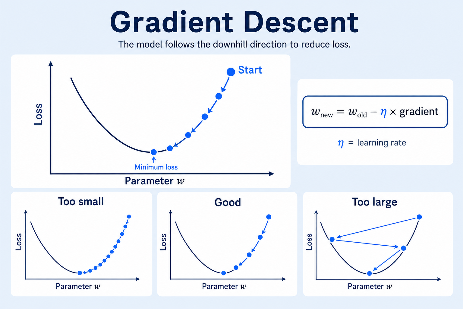
Read one update from right to left

1. Start at the current value of w and measure the curve’s slope there.
2. That slope is the gradient. It points toward increasing loss.
3. Multiply the gradient by the learning rate η to choose the step size.
4. Subtract that step from the old parameter value, moving toward lower loss.
5. Recalculate the gradient at the new point and repeat.

The bottom row shows why learning rate matters:

• Too small: each update helps, but progress is unnecessarily slow.
• Suitable: updates move steadily toward a low-loss region.
• Too large: updates can jump across the valley, oscillate, or even move farther away.

This smooth, one-parameter bowl is a teaching model. A real neural network has many parameters and a high-dimensional loss landscape containing valleys, plateaus, saddle points, noise from mini-batches, and many possible low-loss regions.

A tiny worked example. Suppose our loss function is L(w) = w² (a simple bowl shape, minimum at w = 0), we start at w = 4, and our learning rate is 0.1.

gradient at w=4:  L'(w) = 2w = 2(4) = 8

new w = 4 - 0.1 * 8 = 4 - 0.8 = 3.2

Repeat this a few more times, and w keeps sliding closer and closer to 0 — the point of lowest loss.

Choosing the Learning Rate

The learning rate controls your step size, and getting it wrong breaks training in two very different ways:

Learning rate	What happens
Too small	Training crawls forward painfully slowly, taking far longer than necessary to improve
Too large	Updates overshoot the minimum entirely, and the model can bounce around unstably or fail to improve at all
Just right	Steady, efficient progress toward lower loss

Too small:        Too large:            Just right:
   *. . .              *  →  *              *
    . . .                  ↖   ↗              \
     . . .↘                  *                  \
          minimum       (overshoots wildly)       *  (settles at minimum)

⚠️ Common Mistake A smaller learning rate often makes individual updates less aggressive, but “smaller” is not automatically better. It can make progress too slow for the available training budget. Teams tune the rate and often change it during training with a schedule.

Production Optimization: SGD vs. AdamW SGD and AdamW are both used in real systems; the choice depends on the architecture and task. AdamW tracks moving averages of gradients and squared gradients to scale updates per parameter. It also applies weight decay separately from the gradient-based update. Learning-rate schedules, gradient clipping, precision, batch size, and optimizer settings all interact.

Local Minimum vs. Global Minimum

Real loss landscapes are not one smooth bowl. They contain valleys, flat regions, steep cliffs, and saddle points that slope upward in some directions and downward in others. A local minimum is lower than nearby points; a global minimum is lowest across the whole landscape. Low training loss alone is not the goal—a model must also generalize to suitable validation and test data.

✅ Key takeaway Predict, measure loss, compute gradients, update, and repeat is the core optimization loop. Real LLM training adds data pipelines, batching, distributed computation, checkpointing, learning-rate schedules, evaluation, and often several post-training stages.

Checkpoint: Before moving on, make sure you can answer:

• What does the learning rate control?
• What happens when the learning rate is too small?
• What happens when the learning rate is too large?

---

Part 10 — Linear Algebra: The Language Behind Modern AI

We’ve already used most of linear algebra’s core tools — dot products, matrix multiplication, vectors. This section revisits them at a slightly deeper level, because a few more ideas are needed to understand how attention (the mechanism behind Transformers) actually works.

Linear Transformations

Every time you compute Wx, you’re applying a linear transformation — a way of stretching, rotating, or reshaping a vector’s space while preserving straight lines and the origin’s position. Neural network layers are, quite literally, chains of linear transformations (via W) interleaved with nonlinear bends (via functions like ReLU, from Part 2).

See a matrix transform a vector

The diagram starts with v = [2, 1]. The matrix doubles the x-component and leaves the y-component unchanged, so the output becomes Av = [4, 1].

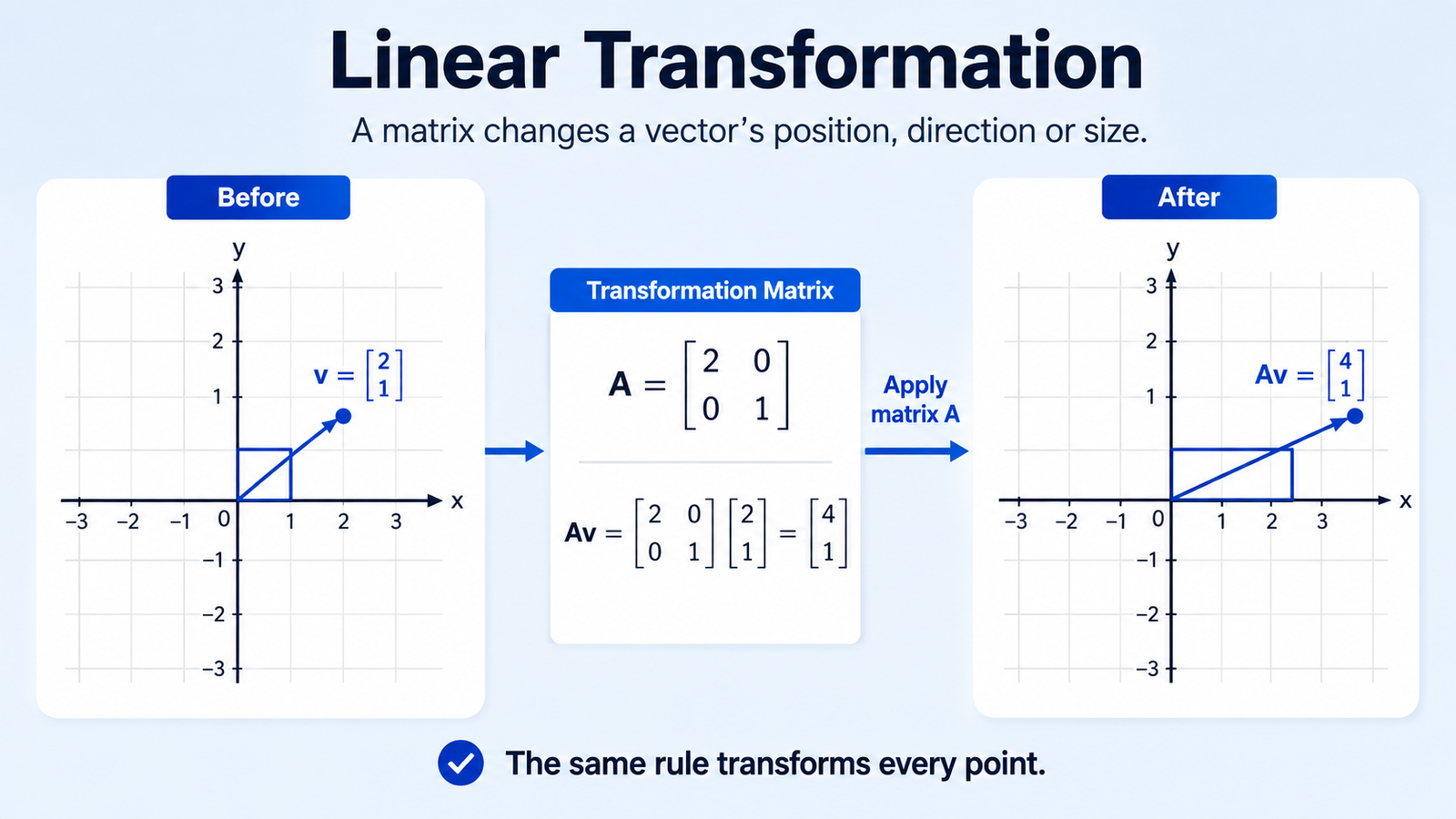
Multiply one output component at a time

A = [2  0]      v = [2]
    [0  1]          [1]

new x = (2 × 2) + (0 × 1) = 4
new y = (0 × 2) + (1 × 1) = 1

Av = [4, 1]

• The first matrix row calculates the new x-component.
• The second matrix row calculates the new y-component.
• Because only x is doubled, the arrow stretches horizontally and changes direction as a result.
• The same matrix rule transforms every input vector consistently.
• A linear transformation always maps the origin to the origin. It can stretch, rotate, reflect, shear, project, or combine these effects, but an ordinary position shift requires an added bias or an affine transformation.

In a neural-network layer, W performs this learned transformation. The layer commonly computes Wx + b, where the bias b adds a shift, and then an activation function introduces nonlinearity.

Eigenvalues and Eigenvectors (Intuition Only)

For a square matrix, an eigenvector is a nonzero direction that the transformation scales without changing that direction; the scale factor is its eigenvalue. Not every matrix has a full set of real eigenvectors, so treat this as intuition rather than a universal picture.

💡 Think about it Picture arrows drawn on a stretchy grid. A linear transformation keeps straight lines straight. Most arrows change direction, while special eigenvector directions only stretch, shrink, or reverse.

You don’t need to calculate these by hand for AI work — but the intuition matters: eigenvectors reveal the “natural axes” along which a transformation acts simply, which underlies techniques for compressing and analyzing high-dimensional data.

Projection and Similarity

A projection takes a vector and finds its “shadow” along another direction — how much of vector A points in the same direction as vector B. This is deeply connected to the dot product from Part 4: the dot product essentially measures how much one vector projects onto another, scaled by their lengths.

Dot product        →  measures alignment between two vectors
Matrix multiplication →  many dot products performed at once, efficiently
Projection          →  measures or maps the component along chosen directions

The Bridge to Attention

Inside most widely used Transformer LLMs, each token’s current representation is multiplied by learned projection matrices to produce Query, Key, and Value vectors. These vectors are recomputed at each layer from the current representations; they are not permanent dictionary entries attached to words.

To figure out how much attention one word should pay to another, the model computes:

$$\text{query} \cdot \text{key}$$

The dot product supplies a compatibility score between a query and key. Attention scales these scores, applies any mask, and uses softmax so the allowed weights for one query add to 1. It then computes a weighted sum of Value vectors. A high score means more influence in that head and layer; it does not by itself explain the model’s final answer.

"The trophy didn't fit in the suitcase because it was too big"

query("it") · key("trophy")   → high dot product  → pay attention here
query("it") · key("suitcase") → lower dot product → pay less attention

🧠 AI Connection Dot products and matrix multiplication form an important core of attention, together with scaling, masking, softmax, weighted sums, multiple heads, and surrounding neural-network layers. The Query, Key, and Value projection matrices are learned through the training loop from Part 9.

We’re not going to unpack attention any further here — that’s a full tutorial of its own, coming later in this series. For now, the important realization is simply this: you already know the mathematics attention is built from.

---

Part 11 — The Big Connection

Let’s stop introducing new mathematics and connect everything into one picture.

REAL WORLD
    ↓
DATA                     (text, images, audio)
    ↓
NUMERICAL REPRESENTATION Part 1
    ↓
TENSORS                  Part 6  (organized values and named axes)
    ↓
FUNCTIONS                Part 2  (transform inputs)
    ↓
VECTORS / MATRICES       Parts 4–5  (represent and transform many values)
    ↓
MODEL PREDICTION
    ↓
PROBABILITY DISTRIBUTION Part 7
    ↓
LOSS                     Part 7  (compare prediction with target)
    ↓
GRADIENT                 Part 8  (how parameter changes affect loss)
    ↓
OPTIMIZATION             Part 9  (update parameters)
    ↓
REPEAT OVER DATA ─────────────────┐
    ↓
TRAINED MODEL  ←──────────────────┘

A Transformer is one possible model architecture inside this loop.
Its attention mechanism uses the linear algebra from Part 10.

Here’s exactly which mathematical idea powers each stage of that chain:

Concept	Section	Role in AI
Numbers	Part 1–2	The raw material everything is built from
Functions	Part 2	The basic unit a neural network is composed of
Coordinate geometry	Part 3	Describes locations, dimensions, boundaries, and distance
Vectors	Part 4	Represent ordered features, movements, gradients, and embeddings
Matrices	Part 5	Transform many values at once (y = Wx + b)
Tensors	Part 6	Organize complex, multi-dimensional real-world data
Probability and statistics	Part 7	Represents uncertainty and summarizes data
Calculus	Part 8	Measures how loss changes with each parameter
Optimization	Part 9	Uses gradients to update parameters
Linear algebra	Part 10	Powers similarity, transformations, and attention

✅ Key takeaway These ideas play different roles and are often combined. Not every AI model uses every technique in exactly the same way, but modern neural networks rely heavily on numerical representation, functions, linear algebra, probability, calculus, and optimization.

Real Numbers From the Original Transformer

The 2017 Attention Is All You Need paper published enough detail for a concrete example. Its base model used:

• representation size d_model = 512;
• 8 attention heads;
• Query and Key size d_k = 64 per head; and
• a feed-forward hidden size of 2,048.

The attention scaling term was therefore:

$$\sqrt{d_k} = \sqrt{64} = 8$$

Dividing dot-product scores by 8 kept their magnitude under better control before softmax. This connects dimensions, square roots, dot products, matrices, and probability in one real published architecture.

Modern GPT and Gemini systems also depend on large tensor and matrix operations, but providers do not publish every internal dimension or parameter count for every proprietary model. We should use published numbers when available and avoid inventing precise ones.

Connections to GPT, Gemini, and Embedding Models

• OpenAI’s GPT-4 report describes a base model trained to predict the next item in a document, followed by post-training. That connects token probabilities, loss, gradients, and optimization. The report does not publish enough detail to calculate GPT-4’s private matrix shapes or parameter count.
• Google’s Gemini report describes models trained jointly across text, images, audio, and video using TPU infrastructure. Those modalities begin with tensors of different shapes, but all require numerical representations and large parallel operations.
• OpenAI documents text-embedding-3-large with a default vector size of 3,072. A 3,072-value FP32 vector needs 3,072 × 4 = 12,288 bytes, or about 12 KB, before database and index overhead. One million raw vectors require about 12.3 GB using decimal units.

---

Part 12 — One Complete Example: What Happens When You Type a Question?

Let’s trace one sentence through this entire pipeline. Suppose you type:

“What is Java?”

into a language model.

Inference — Generating a Response

Here is how the complete inference pipeline maps out visually:

graph TD
    Text["'What is Java?'"] --> Tokenizer["Break into Tokens"]
    Tokenizer --> IDs["Convert to Numerical IDs"]
    IDs --> Embeddings["Look up High-D Vectors"]
    Embeddings --> Layers["Run Repeated Transformer Layers"]
    Layers --> Scores["Produce One Logit per Vocabulary Token"]
    Scores --> Softmax["Convert Logits to Probabilities"]
    Softmax --> Predict["Select or Sample a Next Token"]

The pipeline details:

• TOKENS: A tokenizer breaks the text into model-specific pieces. They may not match whole words, so ["What", "is", "Java", "?"] is only an illustration.
• NUMERICAL IDS: Each token is mapped to a number (an index into a vocabulary).
• VECTORS (embeddings): Each token ID becomes a high-dimensional point/vector (Parts 3–4).
• MATRICES / TENSORS: In a simple single-example picture, the representation has shape (sequence_length, model_dimension). Real serving code usually includes batch and possibly other axes.
• TRANSFORMER LAYERS:
  • ATTENTION: Query-key dot products contribute relevance scores (Part 10).
  • y = Wx + b: Linear transformations reshape the representation (Part 5).
• LOGITS AND PROBABILITIES: A final projection produces one logit per vocabulary token, and softmax converts them into a distribution (Part 7).
• NEXT-TOKEN SELECTION: Decoding selects or samples a token. After "What is Java?", a response might begin with "Java", "It", or another plausible token.

The model appends the selected token and repeats until it reaches a stopping condition.

Every arrow uses tools from this tutorial: tokens become vectors (Parts 3–4), vectors form tensors (Part 6), attention uses dot products (Part 10), transformations use matrices (Part 5), and softmax creates a probability distribution (Part 7).

Training — How the Model Learned to Do This At All

The process above is inference — using an already-trained model. Training brings back calculus and optimization from Parts 8 and 9:

PREDICTION            → the model assigns probabilities to possible next tokens
      ↓
LOSS                  → compare the distribution with the next token observed in training data
      ↓
GRADIENTS (calculus)   → measure how changing parameters changes loss (Part 8)
      ↓
OPTIMIZATION           → update parameters using those gradients (Part 9)
      ↓
                        ... repeat across many batches while evaluating whether
                        the model improves and generalizes

🚀 Why This Matters Inference uses a forward pass to produce outputs. Training also performs that forward pass, then adds loss calculation, backpropagation, and an optimizer update. Backpropagation computes gradients; it does not run the language model “in reverse” to produce text.

---

🎯 You Don’t Need to Fear the Math Anymore

You just walked through numbers, functions, geometry, vectors, matrices, tensors, probability, statistics, calculus, optimization, and linear algebra—and connected them to modern AI.

Here’s the important truth: you don’t need to become a mathematician to build AI. You need what you now have — a working sense of what each piece of mathematics is doing, and why it’s there. That’s a fundamentally different (and far more useful) skill than being able to solve equations by hand.

Here’s the compact mental model to carry forward:

Numbers        represent.
Functions      transform.
Geometry       gives meaning a place, so it can be compared.
Vectors        represent meaning and direction.
Matrices       transform many values at once.
Tensors        organize complex, multi-dimensional data.
Probability    represents uncertainty.
Statistics     summarizes data and reveals variation.
Calculus       measures how things change.
Gradients      show how local parameter changes affect loss.
Optimization   uses gradients to update parameters.
Linear algebra makes large-scale transformation and similarity possible.

And here’s where this journey leads next:

Mathematics
    ↓
Machine Learning
    ↓
Neural Networks
    ↓
Deep Learning
    ↓
Transformers
    ↓
LLMs
    ↓
Generative AI
    ↓
RAG
    ↓
AI Agents

Every one of those future tutorials is going to lean directly on the intuition you built here. When you later read “the attention mechanism computes a weighted sum using query-key dot products,” you won’t just nod along — you’ll actually see the mathematics underneath the sentence. That’s the real win of this tutorial: not memorized formulas, but a lens for seeing exactly what’s happening, every time, under the hood of modern AI.

The mathematics was never the obstacle between you and understanding AI. It was always the map.

Primary References

• Attention Is All You Need
• OpenAI GPT-4 Technical Report
• Google DeepMind Gemini Technical Report
• OpenAI Embeddings Guide
• Google Machine Learning Crash Course
• PyTorch Automatic Differentiation